How to Work with Date and Time in Google Sheets
One of the most common tasks in Google Sheets is filtering or aggregating data by date and time, counting the number of days, and more. This post will cover everything you need to know about working with dates and times in Google Sheets.
A. Basics ➡️
1. How Google Sheets Store Date and Time
2. Time Zone
3. How to Add Dates
4. Calendar Dropdown
5. Date and Time Format
6. Duration Format
B. Date Functions ➡️
Get a date:
TODAY()
DATE(year, month, day)
TO_DATE(value)
DATEVALUE(date_string)
Get date components:
YEAR(date)
MONTH(date)
DAY(date)
WEEKDAY(date, [type])
WEEKNUM(date, [type])
ISOWEEKNUM(date)
Manipulate dates:
EDATE(start_date, months)
EOMONTH(start_date, months)
WORKDAY(start_date, num_days, [holidays])
WORKDAY.INTL(start_date, num_days, [weekend], [holidays])
Count difference between dates and duration:
DATEDIF(start_date, end_date, unit)
DAYS360(start_date, end_date, [method])
NETWORKDAYS(start_date, end_date, [holidays])
NETWORKDAYS.INTL(start_date, end_date, [weekend], [holidays])
YEARFRAC(start_date, end_date, [basis])
C. Time Functions ➡️
Get time:
NOW()
TIME(hour, minute, second)
TIMEVALUE(time_string)
EPOCHTODATE(epoch_time, [unit])
Get time components:
HOUR(time)
MINUTE(time)
SECOND(time)
D. How to Filter by Date and Time with Functions ➡️
1. FILTER
2. QUERY
3. SUMIF(S)/COUNTIF(S)/COUNTUNIQUEIFS
E. Recipes, Tips & Tricks ➡️
1. Get date from datetime
2. Extract Time
3. Combine date and time
4. Get Specific Day
5. Count Days
6. Shift Dates
7. Shift Time
8. Compare Dates
9. Compare Time
10. Convert Date and Time to Text
A. Basics
1. How Google Sheets Stores Date and Time
It’s numbers all the way down.
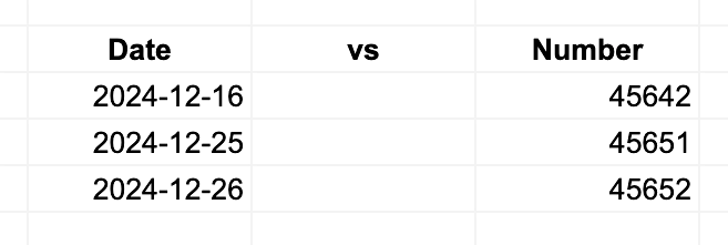
Understanding how Google Sheets stores date and time is crucial for working effectively with them. Google Sheets represents dates as whole numbers, counting the days since December 30, 1899 (not inclusive). For example:
- December 31, 1899, is day 1.
- January 2, 1900, is day 3.
- December 15, 2024, is day 45641.
Time of day is stored as a fraction between 0 and 1, where:
- 0 represents midnight.
- 0.25 is 6:00 AM.
- 0.5 is 12:00 PM, and so on.
If you format a date as a number (which often happens when copying or importing data), it might look like this:
This foundational concept underpins all the techniques we’ll explore later.
2. Time Zone
Another important question is: in what time zone are date and time values stored? This is crucial for both understanding your data and using the NOW() and TODAY() functions, which return the current date and time.
On their own, date and time in Google Sheets are not time zone-aware. This means cell values themselves do not include any time zone information. However, the document as a whole is time zone-aware. When you create a new spreadsheet, it inherits the time zone from your Google account. You can check or change the time zone in the document settings by going to Main Menu -> File -> Settings.
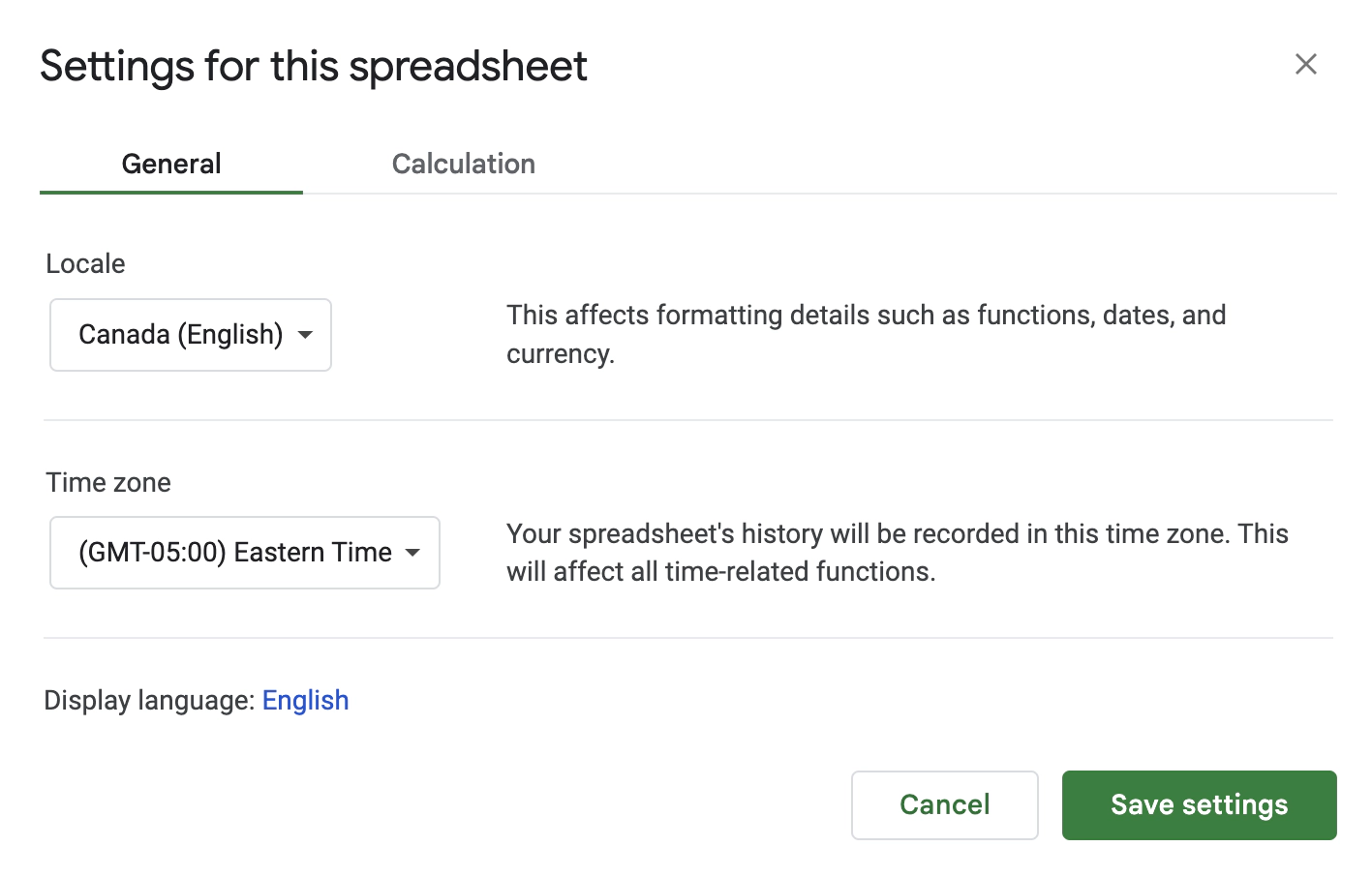
If you change the time zone, the existing cell values will remain the same (except for functions like NOW() and TODAY(), which we’ll cover later). The change simply reinterprets the dates and times as belonging to the new time zone.
Apps Script has its own time zone setting, defined in the appsscript.json file. This is typically the same as the parent document’s time zone (if the script is attached to one). However, if the document and Apps Script use different time zones, their interactions can become confusing: Apps Script will convert the datetime from the spreadsheet into a JavaScript Date object in its own time zone.
3. How to Add Dates
Google Sheets does a good job of recognizing dates when you input them. The specifics depend on your language and location settings. For instance, in most cases, entries like 11/3, 10-12, or 2024-12-15 are identified as dates.
Be cautious with ambiguous formats like 11/3 or 10-12. You might be surprised by which value is treated as the month and which as the day.
Sometimes, Google Sheets can be overzealous and interpret inputs as dates even when they are not.
The issue is that once a value is converted into a date, it becomes a number (as discussed above), and the original text you entered is lost.
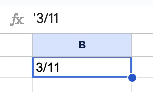
To prevent this, you can add a single quote (') at the beginning of the value. This forces Google Sheets to treat the input as text and bypass automatic date recognition. The single quote will not be displayed in the cell.
4. Calendar Dropdown
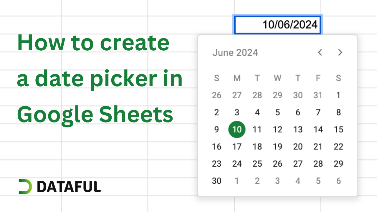
Another convenient way to add a date to Google Sheets is by using a date dropdown. You can learn how to create one in this post or watch this video:
5. Date and Time Format
Since dates and times are stored as numbers, their display depends entirely on formatting. You can present the same date in various ways:
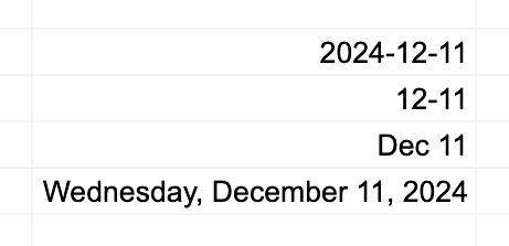
All these cells share the same underlying value but are displayed differently through formatting options:

The exact format options available depend on your document’s locale settings and the format applied prior. To adjust these settings, go to Main Menu -> File -> Settings.
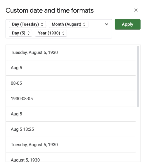
For finer control, you can create a custom date and time format to specify exactly how the data should appear:
6. Duration Format
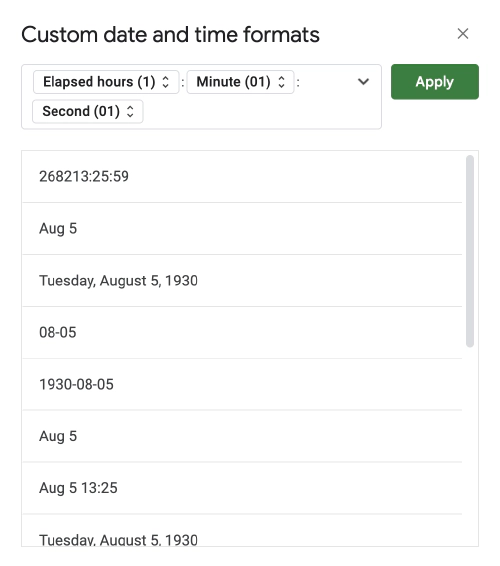
Durations are also stored as numbers, but their display differs based on formatting. To show durations longer than 24 hours, use the Duration format (More formats -> Duration) or set a custom format:
Functions
In this section, we’ll explore different functions for working with dates and times. Some are specialized and complex, so each will include a link to the official documentation for further details.
These are not the only functions available for date and time. Many other functions can handle date/time manipulations, as we’ll see in the recipe section.
B. Date Functions
These are the Google Sheets functions designed specifically for working with dates. However, since dates are essentially numbers behind the scenes, almost any Google Sheets function can be applied to them.
TODAY()
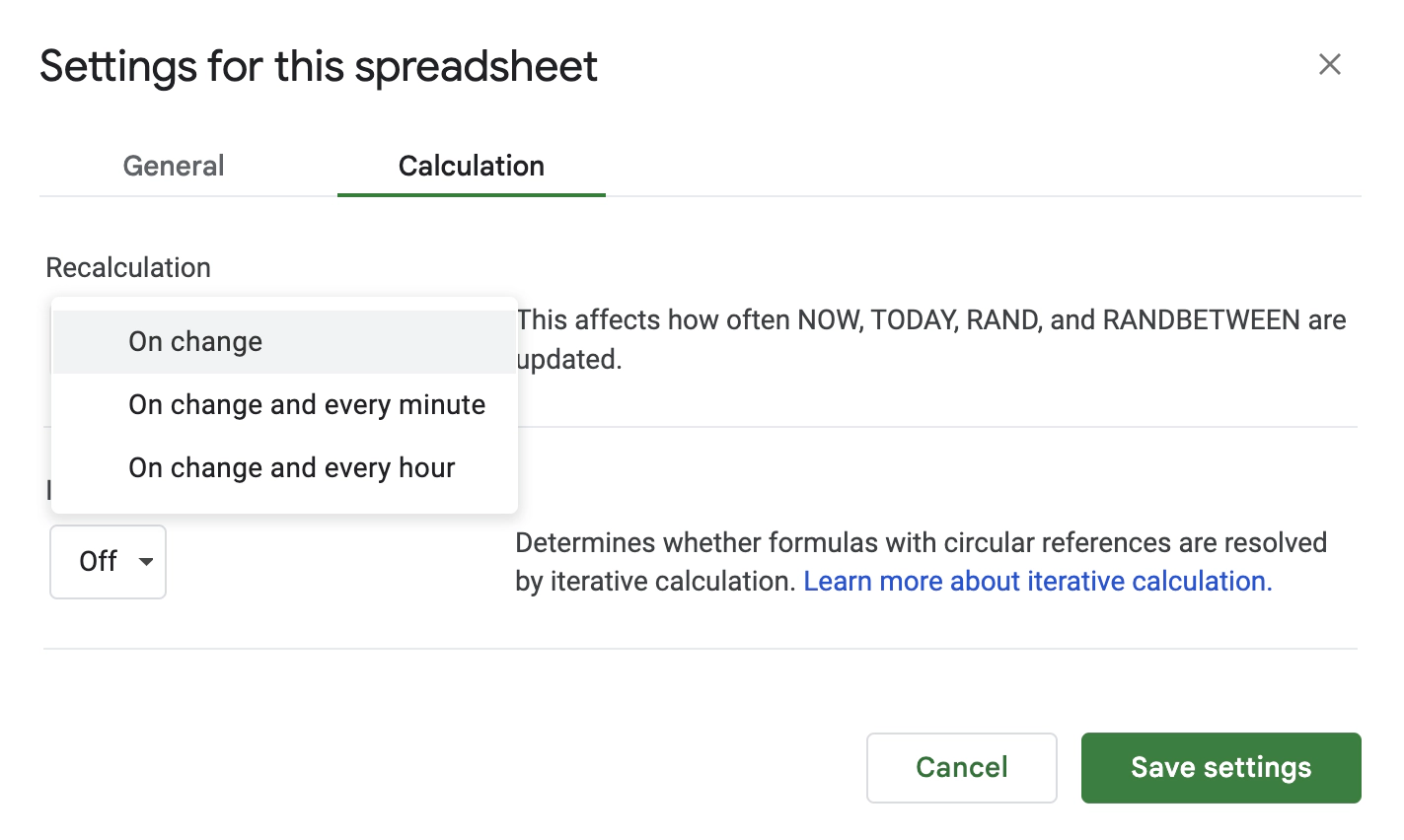
Returns the current date based on the document’s time zone. It recalculates whenever there’s a change in the document or at intervals (e.g., every minute or hour). Adjust recalculation settings in Main Menu -> File -> Settings -> Calculation:
DATE(year, month, day)
Generates a date using the specified year, month, and day. If the month or day exceeds normal limits (e.g., a 15th month or 32nd day), the function adds the overflow to the result:
Example: =DATE(2024, 15, 10) → 2025-03-10
TO_DATE(value)
Converts a serial number or text into a date. Works with numbers where 1 corresponds to 1899-12-31 and increments by days. Text inputs are parsed if they represent valid dates:
=TO_DATE(45000)→2023-03-24=TO_DATE("2024-11-26")→2024-11-26
DATEVALUE(date_string)
Converts a date stored as text into a serial number representing the number of days since 1899-12-31:
Example: =DATEVALUE("2024-11-26") → 45260
The input text must be in a valid date format recognized by Google Sheets.
YEAR(date)
Returns the year of the given date as a four-digit number:
Example: =YEAR(DATE(2024, 11, 26)) → 2024
MONTH(date)
Returns the month of the given date as a number from 1 (January) to 12 (December):
Example: =MONTH(DATE(2024, 11, 26)) → 11
DAY(date)
Returns the day of the month from the given date as a number from 1 to 31:
Example: =DAY(DATE(2024, 11, 26)) → 26
WEEKDAY(date, [type])
Returns the day of the week for the given date as a number. The optional type argument determines the numbering system:
- Type 1 (default): Numbers Sunday as 1 through Saturday as 7.
- Type 2: Numbers Monday as 1 through Sunday as 7.
- Type 3: Numbers Monday as 0 through Sunday as 6.
Examples:
=WEEKDAY(DATE(2024, 11, 26), 1)→3(Tuesday).=WEEKDAY(DATE(2024, 11, 26), 2)→2(Tuesday).=WEEKDAY(DATE(2024, 11, 26), 3)→1(Tuesday).
WEEKNUM(date, [type])
Returns the week number of the year for a date. The optional type argument determines the starting day of the week:
- Type 1 (default): Week starts on Sunday.
- Type 2: Week starts on Monday.
Examples:
=WEEKNUM(DATE(2024, 11, 24), 1)→48(48th week of the year).=WEEKNUM(DATE(2024, 11, 24), 2)→47.=WEEKNUM(DATE(2023, 1, 2), 2)→2(Week 1 starts with January 1st, Sunday, while January 2nd begins Week 2).
ISOWEEKNUM(date)
Returns the ISO 8601 (wiki) week number of the year for a date (weeks start on Monday, and the first week contains January 4).
Example: =ISOWEEKNUM(DATE(2024, 11, 26)) → 48 (48th week of the year).
EDATE(start_date, months)
Returns the date that is the specified number of months before or after the given start date. It maintains the same day of the month or adjusts for month-end dates when necessary.
Examples:
=EDATE(DATE(2024, 11, 26), -3)→2024-08-26(3 months earlier).=EDATE(DATE(2024, 1, 31), 1)→2024-02-29(adjusts for February).
EOMONTH(start_date, months)
Returns the last day of the month, offset by the specified number of months. The offset can be:
- Positive (future months).
- Negative (past months).
- Zero (the current month’s end).
Example: =EOMONTH(DATE(2024, 11, 26), 1) → 2024-12-31
WORKDAY(start_date, num_days, [holidays])
Returns the date after skipping a specified number of working days (excluding weekends and optional holidays). By default this function assumes weekends are Saturday and Sunday.
Example: =WORKDAY(DATE(2024, 1, 1), 10, {DATE(2024, 1, 10)}) → 2024-01-16
WORKDAY.INTL(start_date, num_days, [weekend], [holidays])
Returns a date after a specified number of working days, allowing custom weekend definitions and optional holidays. If num_days is negative, it calculates backward.
-
weekend: Defines weekend days using:
- A string (e.g.,
"0000011"where1marks weekend days like Saturday and Sunday). - A numeric code (e.g.,
1for Saturday-Sunday,2for Sunday-Monday). See the documentation for all codes.
Defaults to Saturday and Sunday.
- A string (e.g.,
-
holidays: A range or array of specific holiday dates to exclude.
Example: =WORKDAY.INTL(DATE(2024, 1, 1), 10, "0000011", {DATE(2024, 1, 10)}) → 2024-01-16 (skips weekends and the specified holiday).
DATEDIF(start_date, end_date, unit)
Calculates the difference between two dates based on the specified unit:
- “Y”: Complete years.
- “M”: Complete months.
- “D”: Total days.
- “MD”: Days, ignoring months and years.
- “YM”: Months, ignoring years.
- “YD”: Days, ignoring years.
Examples:
=DATEDIF(DATE(2024, 1, 1), DATE(2024, 11, 26), "Y")→0(years)=DATEDIF(DATE(2024, 1, 1), DATE(2024, 11, 26), "M")→10(months)=DATEDIF(DATE(2024, 1, 1), DATE(2024, 11, 26), "D")→330(days)
DAYS360(start_date, end_date, [method])
Calculates the number of days between two dates based on a 360-day year (12 months of 30 days each). The optional method parameter determines the calculation convention:
- FALSE (default): U.S. convention.
- TRUE: European convention.
For detailed differences between these methods, refer to the documentation.
Example: =DAYS360(DATE(2024, 1, 1), DATE(2024, 11, 26)) → 325
NETWORKDAYS(start_date, end_date, [holidays])
Returns the number of working days between two dates, excluding weekends (Saturday and Sunday by default) and any optional holidays provided.
Example:
=NETWORKDAYS(DATE(2024, 1, 1), DATE(2024, 1, 31), {DATE(2024, 1, 10)}) → 22 (excludes weekends and the specified holiday)
NETWORKDAYS.INTL(start_date, end_date, [weekend], [holidays])
Returns the number of working days between two dates, with customizable weekend definitions and optional holidays.
- weekend:
- A string (e.g.,
"0000011"for Saturday and Sunday). - A predefined number (e.g.,
1for Saturday-Sunday,2for Sunday-Monday). See the documentation for all codes.
Defaults to Saturday and Sunday.
- A string (e.g.,
- holidays: A range or array of specific holiday dates to exclude.
Example:
=NETWORKDAYS.INTL(DATE(2024, 1, 1), DATE(2024, 1, 31), "0000011", {DATE(2024, 1, 10)}) → 22 (excludes weekends and the specified holiday)
YEARFRAC(start_date, end_date, [basis])
Calculates the fraction of a year between two dates. The optional basis parameter specifies the day count convention:
- 0 (default): 30/360 (U.S. convention).
- 1: Actual/Actual.
- 2: Actual/360.
- 3: Actual/365.
- 4: European 30/360.
Example: =YEARFRAC(DATE(2024, 1, 1), DATE(2024, 11, 26)) → 0.902778 (fraction of the year)
C. Time Functions
Google Sheets provides functions specifically designed for working with time. These functions allow you to manipulate, calculate, and format time values efficiently.
NOW()
Returns the current date and time based on the document’s time zone. The value updates dynamically whenever changes occur in the document or according to the recalculation settings (see above).
Example: =NOW() → 2024-11-26 14:35:12 (current date and time)
TIME(hour, minute, second)
Returns a time value constructed from the specified hour, minute, and second. The result represents a fraction of a 24-hour day.
Example: =TIME(14, 35, 12) → 14:35:12
TIMEVALUE(time_string)
Converts a time stored as text into a decimal number that represents the fraction of a 24-hour day.
Example: =TIMEVALUE("14:35:12") → 0.6075 (time as a fraction of 24 hours)
EPOCHTODATE(epoch_time, [unit])
Converts an epoch timestamp into a date and time (wiki).
- epoch_time: The number of seconds, milliseconds, or microseconds since
1970-01-01 00:00:00 UTC. - unit (optional): Specifies the unit of the epoch time:
1(default): Seconds.2: Milliseconds.3: Microseconds.
Example: =EPOCHTODATE(1698452112, "s") → 2023-10-27 12:01:52
HOUR(time)
Returns the hour (0–23) from a given time value.
Example: =HOUR(TIME(14, 35, 12)) → 14
MINUTE(time)
Returns the minute (0–59) from a given time value.
Example: =MINUTE(TIME(14, 35, 12)) → 35
SECOND(time)
Returns the second (0–59) from a given time value.
Example: =SECOND(TIME(14, 35, 12)) → 12
D. How to Filter by Date & Time with Functions
This section explains how to use dates in various aggregation and filtering functions.
The comparison range must contain dates recognized by Google Sheets. If the dates are stored as text, comparisons may not work correctly. To confirm a cell contains a proper date, double-click it—this should display a dropdown calendar.
1. FILTER
You can use dates directly in the FILTER function by applying logical operators (=, <>, <, >, <=, >=).
Example: =FILTER(B1:B6, A1:A6=DATE(2024, 11, 02))
Logical operators also work with complex conditions.
Filtering by Month
To filter data by month, combine both MONTH and (optionally) YEAR to handle multi-year datasets: =FILTER(B1:B6, MONTH(A1:A6)=MONTH(C1), YEAR(A1:A6)=YEAR(C1)).
Filtering Without Time
When the same date includes different times, comparisons may produce unexpected results. Use INT to strip the time portion: =FILTER(B1:B6, INT(A1:A6)=INT(C1)).
2. QUERY
The QUERY function allows filtering data using SQL-like syntax (documentation).
Using Dates
To filter by a date, pass it as text in YYYY-MM-DD format and prepend it with the DATE keyword: =QUERY(A1:B6, "SELECT B WHERE A = DATE '2024-11-02'")
You can use all standard logical operators: =, <>, <, >, <=, >=.
Using Dates from Cells
To use a date stored in a cell, convert it to text: =QUERY(A1:B6, "SELECT B WHERE A = DATE '" & TEXT(D1, "yyyy-MM-dd") & "'")
Time Considerations
Unlike FILTER, the QUERY function compares exact dates, so there’s no need to strip time from the values.
Filtering by Time or Datetime
The QUERY function also supports the TIMEOFDAY and DATETIME keywords for filtering by time and combined date-time values, respectively.
QUERY guesses the data type in columns, which can lead to unexpected results. Ensure the data in the columns you are filtering by is consistent in format. For example, if most dates in a column lack a time component and you filter by a datetime value, the results may not match your expectations.
3. SUMIF(S) / COUNTIF(S) / COUNTUNIQUEIFS
These functions allow you to compute aggregate statistics like sums, counts, and unique counts based on some criteria:
SUMIF(range, criteria, [sum_range])SUMIFS(sum_range, criteria_range1, criteria1, [criteria_range2, criteria2, ...])COUNTIF(range, criteria)COUNTIFS(criteria_range1, criteria1, [criteria_range2, criteria2, ...])COUNTUNIQUEIFS(range, criteria_range1, criteria1, [criteria_range2, criteria2, ...])
All these functions use similar syntax: criteria are applied to a range. Dates can be used as criteria directly. Examples:
-
Sum values between two dates (inclusive):
=SUMIFS(B1:B6, A1:A6, ">=" & DATE(2024, 11, 01), A1:A6, "<=" & DATE(2024, 11, 02)) -
Count items that fall between two dates (exclusive):
=COUNTIFS(A1:A6, ">" & DATE(2024, 11, 01), A1:A6, "<" & DATE(2024, 11, 02)) -
Count unique values in column B for a specific date in column A:
=COUNTUNIQUEIFS(B1:B6, A1:A6, DATE(2024, 11, 01))
These functions support all comparison operators: = (you can omit the = sign), <>, <, >, <=, and >=.
Handling Date and Time Components
When working with datetime values, you may need to explicitly manage the date or time components:
-
Compare by date only (strip time):
=SUMIFS(B1:B6, A1:A6, ">=" & INT(C1), A1:A6, "<=" & INT(D1)) -
Compare by time only (strip date):
=SUMIFS(B1:B6, A1:A6, ">=" & MOD(C1, 1), A1:A6, "<=" & MOD(D1, 1)) -
Filter by specific date in datetime data (using date and date + 1):
=SUMIFS(B1:B6, A1:A6, ">=" & C1, A1:A6, "<" & (C1 + 1))
(Note: The upper boundary is exclusive.)
E. Recipes, Tips & Tricks
This section covers common operations with dates and times in Google Sheets. Since dates and times are stored as numbers, many techniques involve standard numeric operations.
1. Get Date from Datetime
To extract the date component from a cell containing both date and time, round it down using =INT(datetime).
This is particularly useful for comparisons, such as checking if two dates are equal.
2. Extract Time
To extract the time component from a datetime value, use: =MOD(datetime, 1).
3. Combine Date and Time
To combine a date and a time, simply add them together:
=DATE(2024, 11, 26) + TIME(14, 43, 55) → 2024-11-26 14:43:55.
4. Get Specific Day
First Day of the Month
- Using
DATE:
=DATE(YEAR(date), MONTH(date), 1) - Using
EOMONTH:
=EOMONTH(date, -1) + 1
(Gets the last day of the previous month and adds one.)
Last Day of the Month
=EOMONTH(date, 0)
Monday of a Week
=date - WEEKDAY(date, 3)
(Returns the Monday of the week for the given date.)
First Day of the Year
=DATE(YEAR(date), 1, 1)
Last Day of the Year
=DATE(YEAR(date), 12, 31)
5. Count Days
Difference Between Two Dates
=A1 - A2
If the first date is later than the second, the result is positive; otherwise, it’s negative.
Count Business Days in a Period
-
Using
NETWORKDAYS:
=NETWORKDAYS(DATE(2024, 1, 1), DATE(2024, 1, 31), {DATE(2024, 1, 10), DATE(2024, 1, 11)})
(Assumes Monday to Friday as business days and excludes the holidays 2024-01-10 and 2024-01-11.) -
Using
NETWORKDAYS.INTL:
=NETWORKDAYS.INTL(DATE(2024, 1, 1), DATE(2024, 1, 31), "0000001", {DATE(2024, 1, 10), DATE(2024, 1, 11)})
(Treats Saturday as a business day in addition to Monday to Friday.)
6. Shift Dates
Add or Subtract Days
- Add days:
=A1 + 7 - Subtract days:
=A1 - 3
Get Date After a Number of Business Days
-
Using
WORKDAY:
=WORKDAY(DATE(2024, 1, 1), 10, {DATE(2024, 1, 10)})
(Assumes Monday to Friday as business days and skips the holiday 2024-01-10.) -
Using
WORKDAY.INTL:
=WORKDAY.INTL(DATE(2024, 1, 1), 10, "0000001", {DATE(2024, 1, 10)})
(Treats Saturday as a business day in addition to Monday to Friday.)
7. Shift Time
To add time to a date in A1:
- Add hours:
=A1 + <number_of_hours>/24 - Add minutes:
=A1 + <number_of_minutes>/24/60 - Add seconds:
=A1 + <number_of_seconds>/24/3600 - Shift an hour earlier:
=A1 - 1/24
8. Compare Dates
Dates support standard comparison operators:
- Equality:
=A1=A2(checks if the dates are the same). - Inequality:
=A1<>A2(checks if the dates are different). - Greater than:
=A1>A2(checks if the first date is after the second). - Greater than or equal to:
=A1>=A2(checks if the first date is after or equal to the second). - Less than:
=A1<A2(checks if the first date is before the second). - Less than or equal to:
=A1<=A2(checks if the first date is before or equal to the second).
If the data includes a time component and you want to compare only the dates, strip the time using:
=INT(A1)=INT(A2)
9. Compare Time
Time values support standard comparison operators:
- Equality:
=A1=A2(checks if the times are the same). - Inequality:
=A1<>A2(checks if the times are different). - Greater than:
=A1>A2(checks if the first time is later than the second). - Greater than or equal to:
=A1>=A2(checks if the first time is later than or equal to the second). - Less than:
=A1<A2(checks if the first time is earlier than the second). - Less than or equal to:
=A1<=A2(checks if the first time is earlier than or equal to the second).
If the data includes a date component and you want to compare only the times, strip the dates using:
=MOD(A1, 1)=MOD(A2, 1)
10. Convert Date and Time to Text
You can convert a date or time to a string in a required format using the TEXT(A1, <format>) function (documentation). The format argument includes placeholders for various date and time components (e.g., d for a one- or two-digit day of the month, mmmm for the full name of a month). The formatting options and language depend on the document’s locale. For the full list of placeholders, see the documentation.
| Example | Format | Comment |
|---|---|---|
| 2/31/24 | m/d/yy |
US style with the month first and no leading zeros |
| February 2, 2024 | mmmm d, yyyy |
Full month name, day, and year with leading zeros |
| 01-01-2024 | dd-mm-yyyy |
Day, month, year with leading zeros, separated by dashes |
| 2024-01-01 | yyyy-mm-dd |
ISO 8601 date format |
| Nov 2024 | mmm yyyy |
Abbreviated month and full year |
| Monday, January 1 | dddd, mmmm d |
Full day of the week and month names |
| 1/1/2024 14:30 | m/d/yyyy h:mm |
Date with 24-hour time |
| 2:30 PM | h:MM AM/PM |
12-hour time with AM/PM |
| 02:30 | HH:MM |
24-hour time with leading zero |
| 14:30:45 | HH:MM:SS |
24-hour time with seconds |
| 2:30 | h:MM |
24-hour time without leading zeros |
| 2 PM | h AM/PM |
Hour only, 12-hour format with AM/PM |
| 14 | HH |
Hour only, 24-hour format |
| 2024-11-28T09:12:36 | yyyy-mm-ddThh:mm:ss |
ISO 8601 date and time format without timezone information * |
* As noted above, dates in Google Sheets are not timezone-aware. If you need timezone information, you must manually add your timezone shift (e.g., "-05:00" or "Z") to the output of the TEXT function. For example:
=TEXT(A1, "yyyy-mm-ddThh:mm:ss") & "-5:00"
Conclusion
Google Sheets offers powerful tools for working with dates and times, from simple calculations to advanced filtering and formatting. By understanding how dates and times are stored and leveraging the functions covered in this guide, you can efficiently manage and analyze your data.
If you have your own tips, tricks, or recipes for working with dates and times, feel free to share them. Got questions or need help with a specific use case? Let us know—we’d be happy to help!