Highlight Duplicates in Google Sheets: A Step-by-Step Guide
When working with data in Google Sheets, it’s common to need to identify duplicates. Follow these steps to highlight duplicates using conditional formatting and a custom formula.
1. Select the Range
First you need to select the range that you need to check for duplicates. If the range is very large you can skip this step and input it later.
2. Open Conditional Formatting Panel
Access the conditional formatting panel either by right-clicking on the selected range, choosing View more cell actions, and then Conditional formatting. Alternatively, via the main menu: Format → Conditional Formatting.
3. Create Conditional Formatting Rule with a Custom Formula
Following step #2, you’ll either see a list of existing conditional formatting rules or be directed to create a new rule. If presented with a list, click + Add another rule.
Ensure the conditional formatting applies to the correct range, adjusting manually if necessary, then apply a custom formula: select Format cells if … → Custom formula is (found at the bottom).
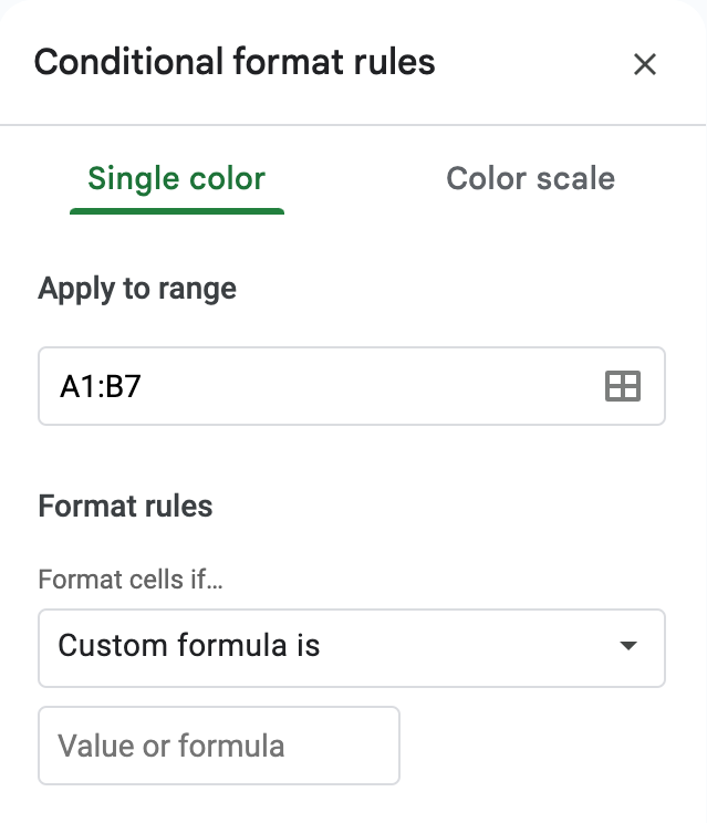
Use a formula like the one below:
=COUNTIF([range with duplicates], [address of top left cell in range]) > 1
This formula counts the occurrences of each cell value within the specified range, highlighting the cell if the count exceeds 1.
The exact addresses in the formula will vary based on your spreadsheet’s layout and your goals. Below are common variations of the formula to highlight duplicates (assuming data is in the range A1:B7):
-
Across all columns in the range:
=COUNTIF($A$1:$B$7, A1) > 1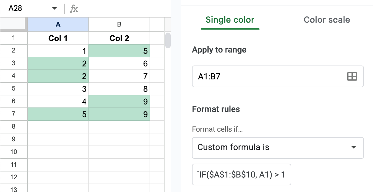
Highlight duplicates across all columns together -
Across all rows of the given columns:
=COUNTIF($A:$B, A1) > 1. This is a preferred approach, especially if you expect data to grow - akin to choosing an optimal size for a named range.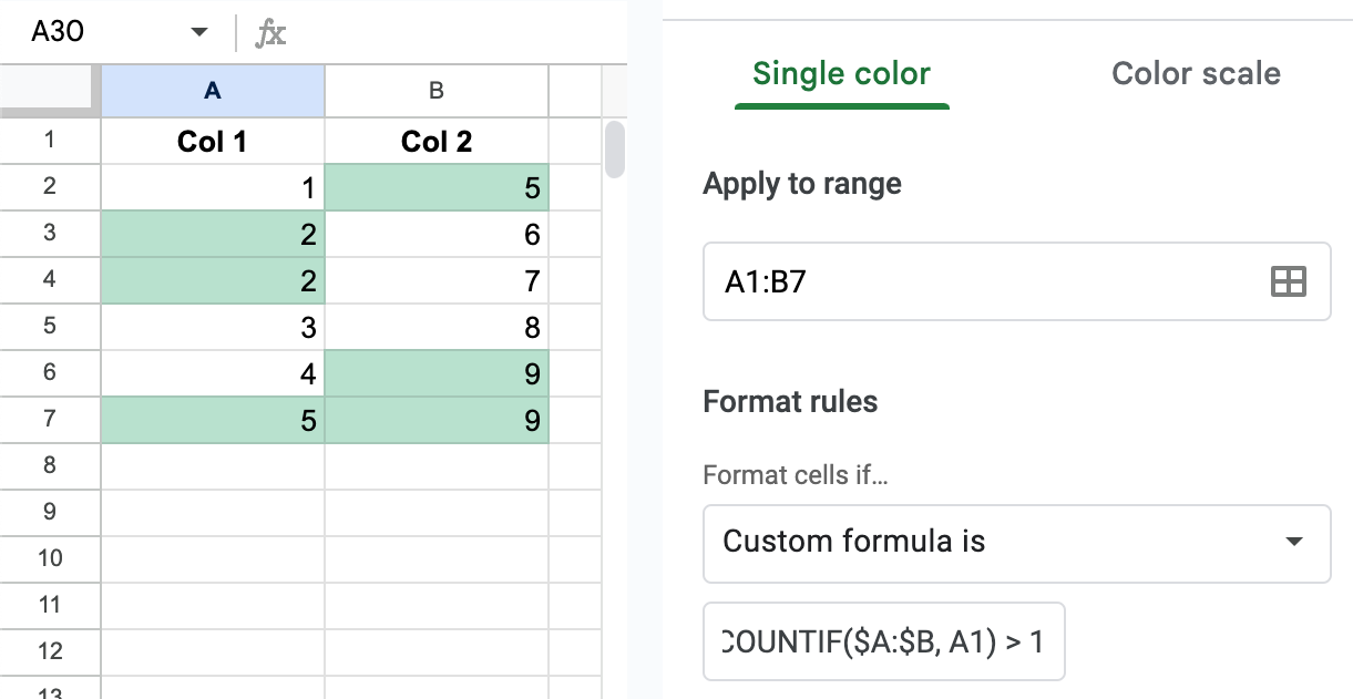
Highlight duplicates across all rows of all columns together -
In each column of the range independently:
=COUNTIF(A$1:A$7, A1) > 1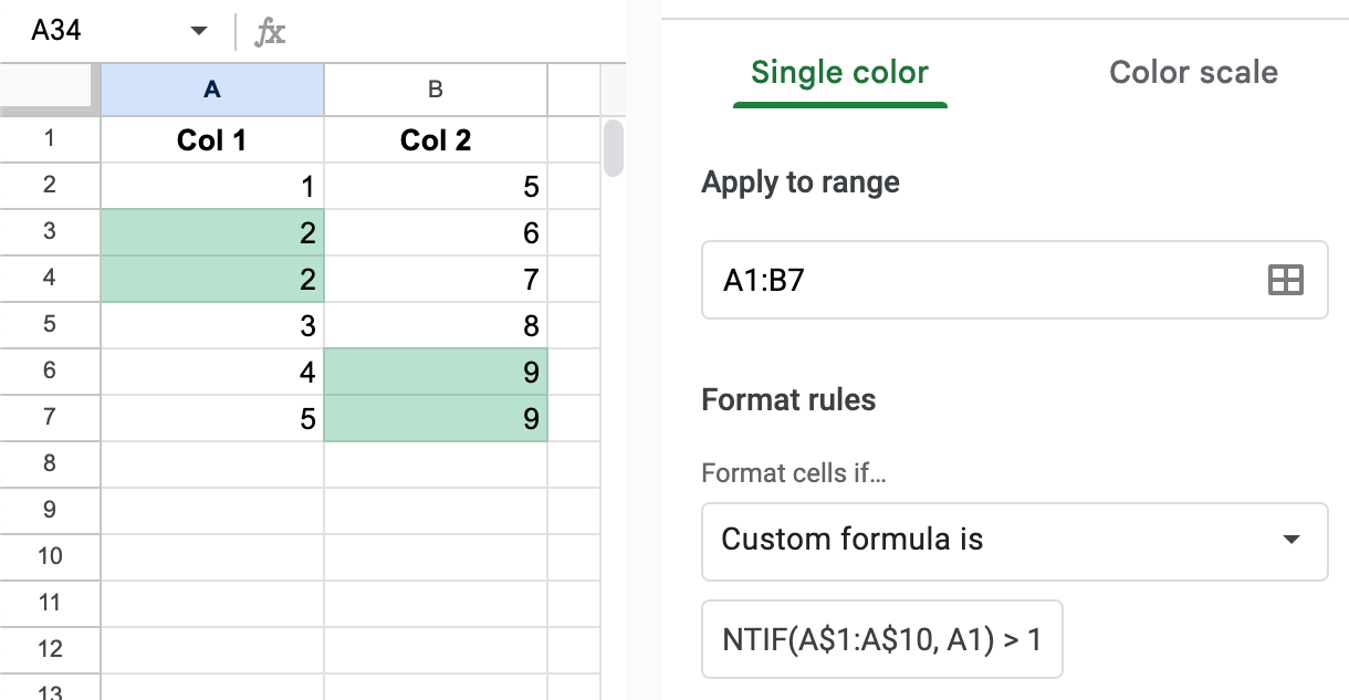
Highlight duplicates in each column of the range independently -
Highlight the entire row if there’s a duplicate in column A:
=COUNTIF($A:$A, $A1) > 1. Apply this rule to the entire range (all columns) you wish to highlight.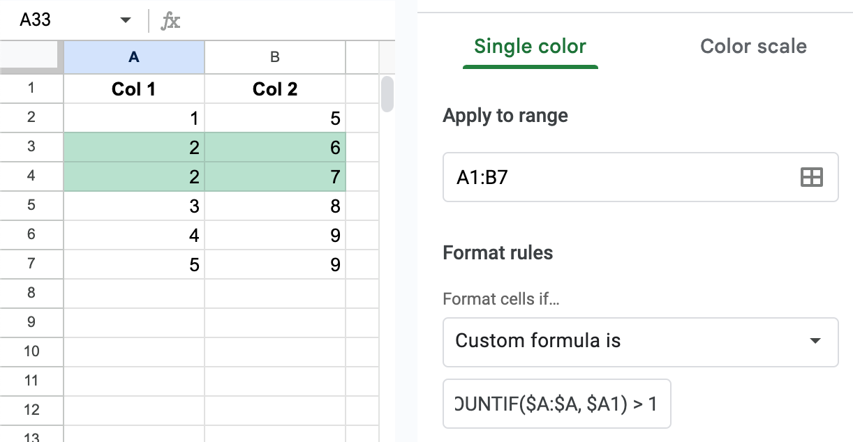
Highlight the entire row if there’s a duplicate in column A -
Highlight after a specific count of duplicates:
=COUNTIF($A:$B, A1) > 2. Use your threshold instead of 2 here.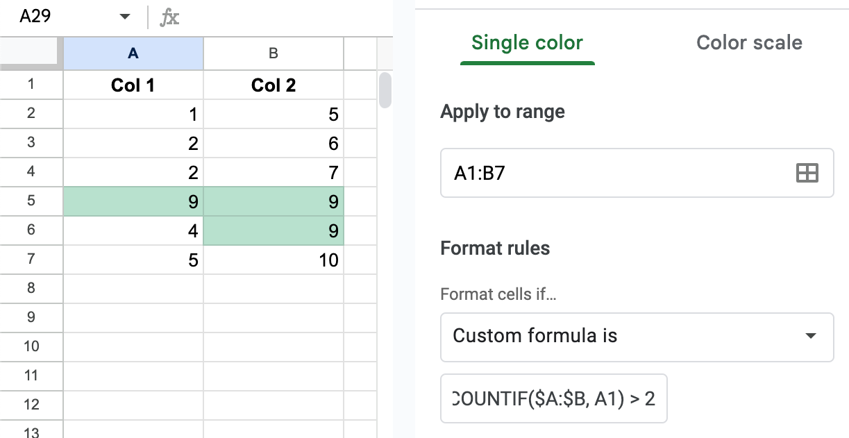
Highlight after a specific count of duplicates
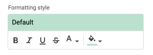
4. Customize Formatting
Customize the formatting of the highlighted duplicates.
5. Save
Save your conditional formatting rule.
In this guide, we’ve outlined a step-by-step approach to highlighting duplicates in Google Sheets using conditional formatting and custom formulas. Mastering these steps allows for more efficient data handling, making it easier to spot and rectify duplicate entries.