Multiple Selection Dropdowns in Google Sheets

Have you ever wished you could select multiple options in Google Sheets dropdowns? Well, now you can! In August 2024, Google introduced multiple-selection dropdowns. In this post, we will look at how to create them, how they work, and how to use them in formulas.

Video version of the guide:

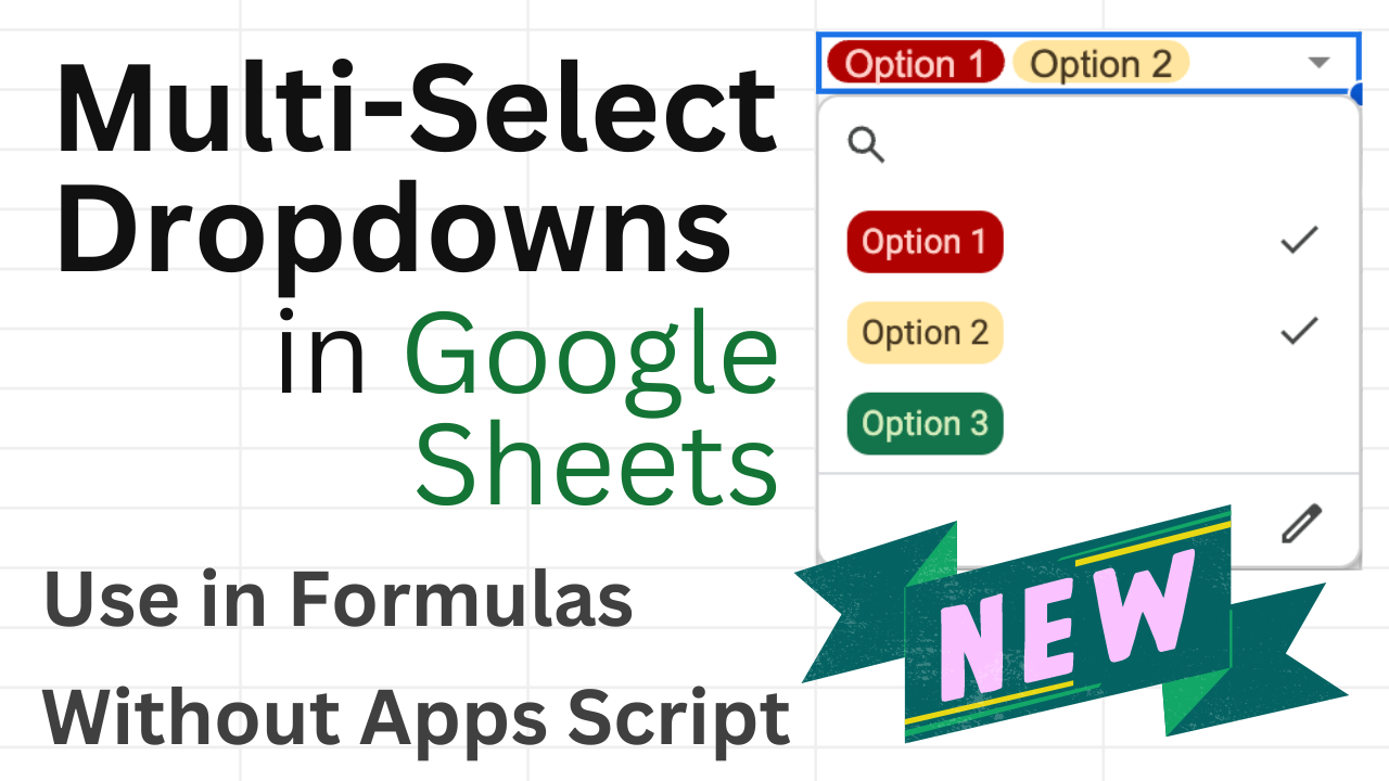
Create Multi-Select Dropdown

To create multi-selection dropdowns, head to the Main Menu -> Insert -> Dropdown, and enable “Allow multiple selections”:

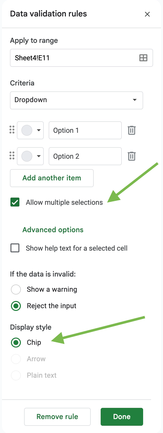
Note that this only works with chip-style dropdowns; other options are disabled.

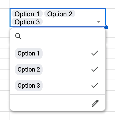
You can enable text wrapping to get the most out of these dropdowns.

Use Dropdowns in Formulas

Under the hood, these multi-select dropdowns join all selected values with a comma and space separator, for example, Option 1, Option 2. Knowing this, you can use them in formulas.

First, let’s check if a value is selected: =ISNUMBER(FIND(<dropdown option>, <dropdown cell>))

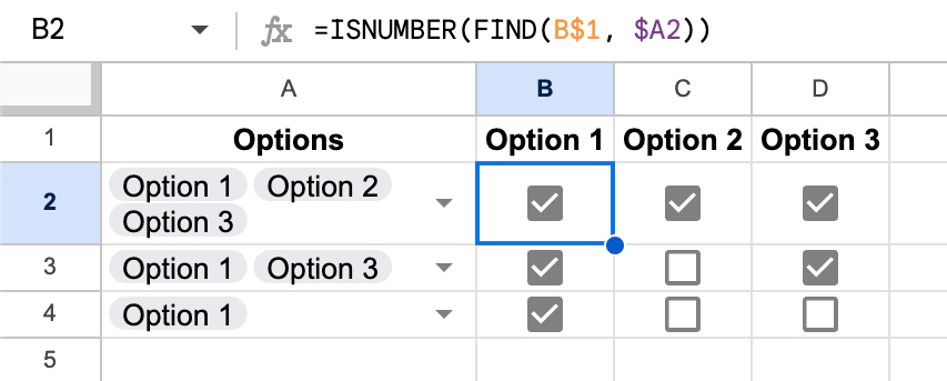
For this, we’ll create columns for the employees and use the FIND function. FIND returns the position of text or an error if it’s not found. Wrapping it with ISNUMBER gives us a true or false value, which we can then convert to a checkbox.

Next, let’s split the selected items into individual cells using the SPLIT function: =IFERROR(SPLIT(<dropdown cell>, ", ", false))

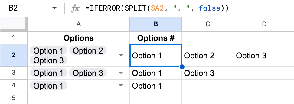
It accepts the value we want to split, then the separator, in this case, it is a comma and a space, and whether to split by each symbol in the separator or use it as a whole; here we want to use false. Wrapping it with IFERROR ensures there are no issues with empty dropdowns.

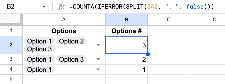
Finally, to count the selected values, we’ll use the previous formula and wrap it in COUNTA, which counts non-empty values in a provided range: =COUNTA(IFERROR(SPLIT(<dropdown cell>, ", ", false)))

---

How will you use these multi-select dropdowns in your spreadsheets? Let me know in the comments.