Dropdowns in Google Sheets: Complete Guide

Dropdowns are a powerful Google Sheets feature that allows you to choose a cell value from a predetermined list of options. In this guide, we will cover:

1. Why use dropdowns
2. How to create a dropdown
3. Dropdown settings
     a. Display styles
     b. What to do if data is invalid
     c. Help text
     d. Coloring
4. Limitations of dropdowns
5. Best practices when using dropdowns
     a. Use dropdowns from a range
     b. Use named ranges
     c. Sort dropdown options
     d. Use hierarchical names

1. Why Use Dropdowns

Dropdowns bring three main benefits:

1. They make the data more consistent: it is much harder to make a mistake when you choose an option instead of typing it in.
2. Input data faster: choosing an option is much faster than typing it in.
3. Visualize data: dropdowns allow you to change the background of a cell based on the value. Colors help distinguish different data points and highlight those requiring attention.

2. How to create a dropdown

1. Open the data validation sidebar. There are several ways to get there:

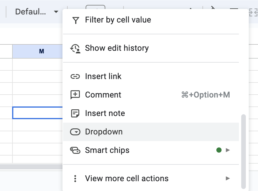
   A. The context menu: Select the cells -> Right click -> Dropdown:

   

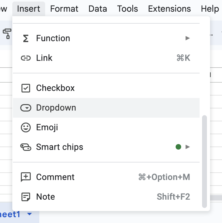
   B. The main menu: Select the cells -> Main Menu -> Insert -> Dropdown:

   

   C. Regular data validation: select the cells where you need a dropdown and either:

   • Right click -> View more cell actions -> Data validation, or
   • Main Menu -> Data -> Data validation.

   Then click on the + Add rule button.

2. Choose the type of a dropdown:

   A. static (default) – you list all dropdown options in the data validation interface.
   B. from a range – dropdown options are pulled from a specified range.

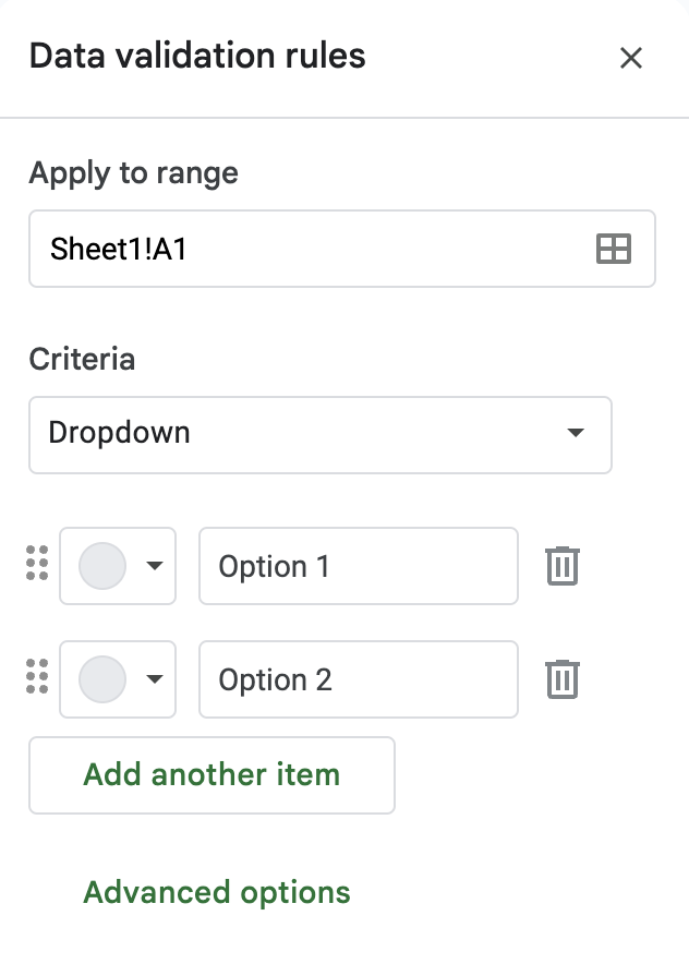
3. For a static dropdown: specify options you want to see in the dropdown.

   

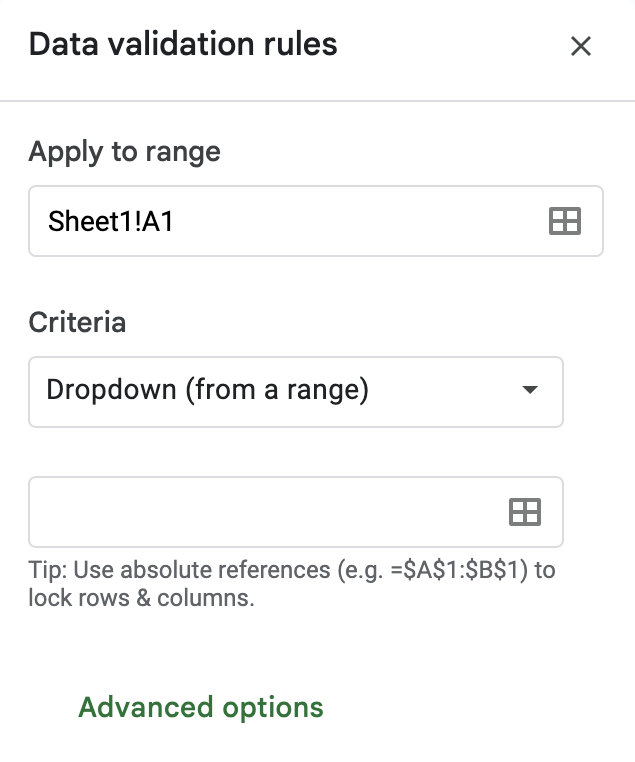
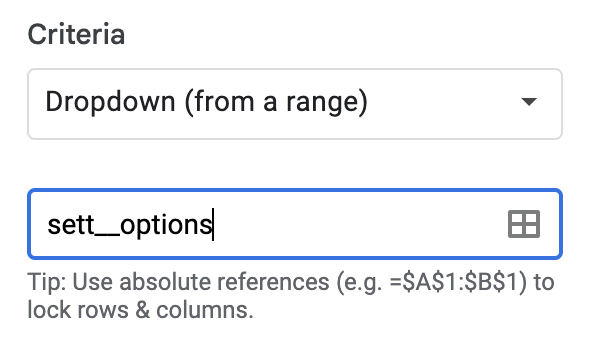
   For a dropdown from a range: type in or select the range that contains the options. You can use named ranges (it is recommended; see best practices for dropdowns).

   

3. Dropdown Settings

Dropdowns have a variety of settings, most of which you can access via Advanced options.

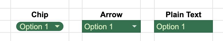
A. Display Style

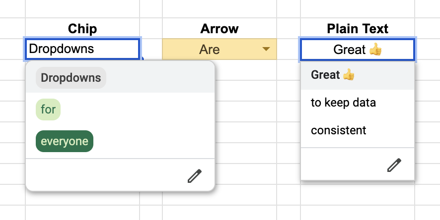
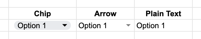
Dropdowns come in three styles: a chip, arrow, or plain text. Here they are side by side (without coloring):

These styles differ only in their appearance; there is no functional difference. It’s up to you which one you like the most. Still, there are some rules of thumb on which ones to choose:

1. Chip or arrow as a default. I mostly use arrows as they color better (see below) and are easier to read.

2. Plain text if you have many dropdowns, for example, in every row or several columns. Using other styles creates visual noise.

B. Invalid Data: Reject or Warn

This setting tells the spreadsheet what to do if the user’s input is invalid (not one of the options):

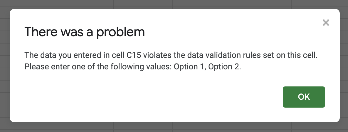
1. Reject the input: invalid data is not saved, and the user will see an error message:

   

   It doesn’t 100% prevent invalid entries. Users can still copy-paste invalid values.
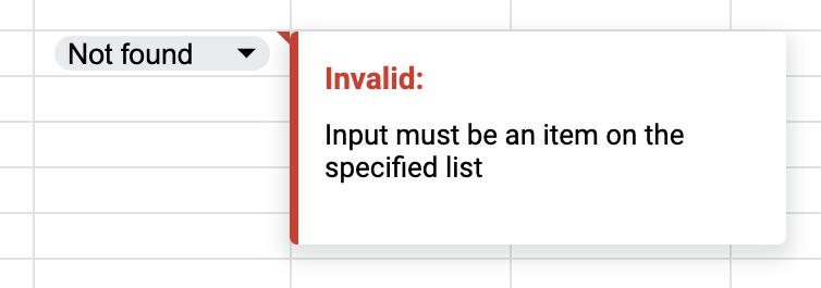
2. Show a warning: the input will be saved, but you will see a red triangle in the top right corner of the cell. If you hover over it, you will see an explanation.

   

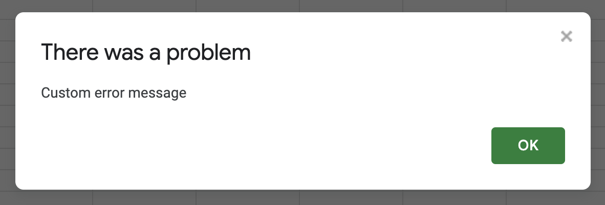
C. Help Text

Message to display to the user if the value is invalid:

Surprisingly, it works only with the reject input option. If you select the “show a warning” option, the error message when you hover over the cell will be generic.

D. Coloring Dropdowns

A natural extension of dropdowns is to add color to them. It is especially useful when you have a limited set of items like statuses, types, grades, etc.

There are two ways to color a dropdown option based on its value: with conditional formatting or data validation settings.

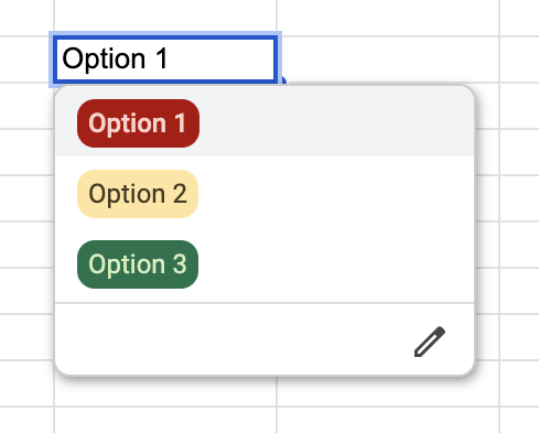
Via Dropdown Settings

This method is relatively new. Now you can assign a background color to any dropdown option in any display style:

This is how the result will look in different styles:

Here lies the most significant difference between the display styles: only chips show the background color in the dropdown:

These settings are the best option when you use a static dropdown and need to color many options. It is much faster than doing the same via conditional formatting.

Conditional Formatting

The second way to color dropdown options is by using conditional formatting. You can create conditional formatting rules of different levels of complexity, from the simplest “Text is exactly” to a flexible and extensible color-coding system in Google Sheets.

Benefits of conditional formatting compared to the dropdown settings:

1. You can move the coloring settings to a separate sheet and apply them anywhere in the spreadsheet.
2. Control the font color and style.
3. Use more complex rules thanks to custom formulas in conditional formatting.

4. Limitations of Dropdowns

Dropdowns in Google Sheets have three main limitations:

1. They work only one way. If you were to change dropdown options to update spelling or remove options, the data that contained those options would not change. You will have to do it manually. Until then, it will be marked as invalid.

2. You can choose only one option per cell. You have to use multiple cells to approximate selecting multiple values from a dropdown.

3. There are no dependent dropdowns out of the box. You still can do it, but the setup will be more complex and has its limitations.

5. Best Practices

Follow these best practices to get the maximum out of your dropdowns.

A. Use Dropdowns From a Range

Static dropdowns work well under three conditions:

1. You have a short list of options.
2. The list does not change.
3. You use it only on at most a couple of different sheets.

Dropdowns from a range are much more robust for all other cases: you can set the options in one place and add new options easily.

B. Use Named Ranges

When creating a dropdown, choose Dropdown (from a range) and use a named range instead of coordinates. Having done that, you can easily extend the list of options, move it, and use it in multiple places.

C. Sort Dropdown Options

Sorting dropdown options in a specific order makes it easier to work with them. Some examples of the sorting approaches:

1. Alphabetically: if you have many options that you use equally often.
2. Most frequently used at the top: if certain items are used more frequently than others.
3. According to their internal logic or sequence: statuses of orders, applications, etc.

In this case, keeping dropdown options in a named range is especially handy.

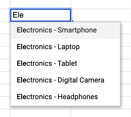
D. Use Hierarchical Names

If you have many options in a dropdown and they belong to specific categories, put the categories at the beginning of the option. It will make sorting more logical and simplify manual selection and search.

---

You now have the know-how to create dropdowns in Google Sheets, customize their settings, and apply best practices for improved data management and consistency.