You often need to sort rows by multiple columns simultaneously to review and analyze the data more efficiently. It is easy to do in Google Sheets with any of these four methods:
Using these techniques, you can order by any criteria and data type, such as date, alphabet, and number.
Video guide:
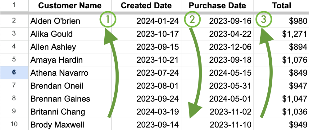
Before sorting the data using any technique, ensure that the data is appropriately formatted. Most importantly, format dates as dates and numbers as numbers. Otherwise, if some cells in a row are in different formats, they will be sorted differently. For example, the sort order of 9 and 10 will differ depending on whether they are formatted as numbers or plain text.
1. Advanced Sorting for Static Data
Google Sheets allows you to sort a range by multiple criteria via so-called advanced sort. It works well when your data is static: you can sort it and forget it.
Select the range you want to sort. Select the whole sheet if you need to sort all the data.
Select the header row as well; it will make sorting easier in step #3.
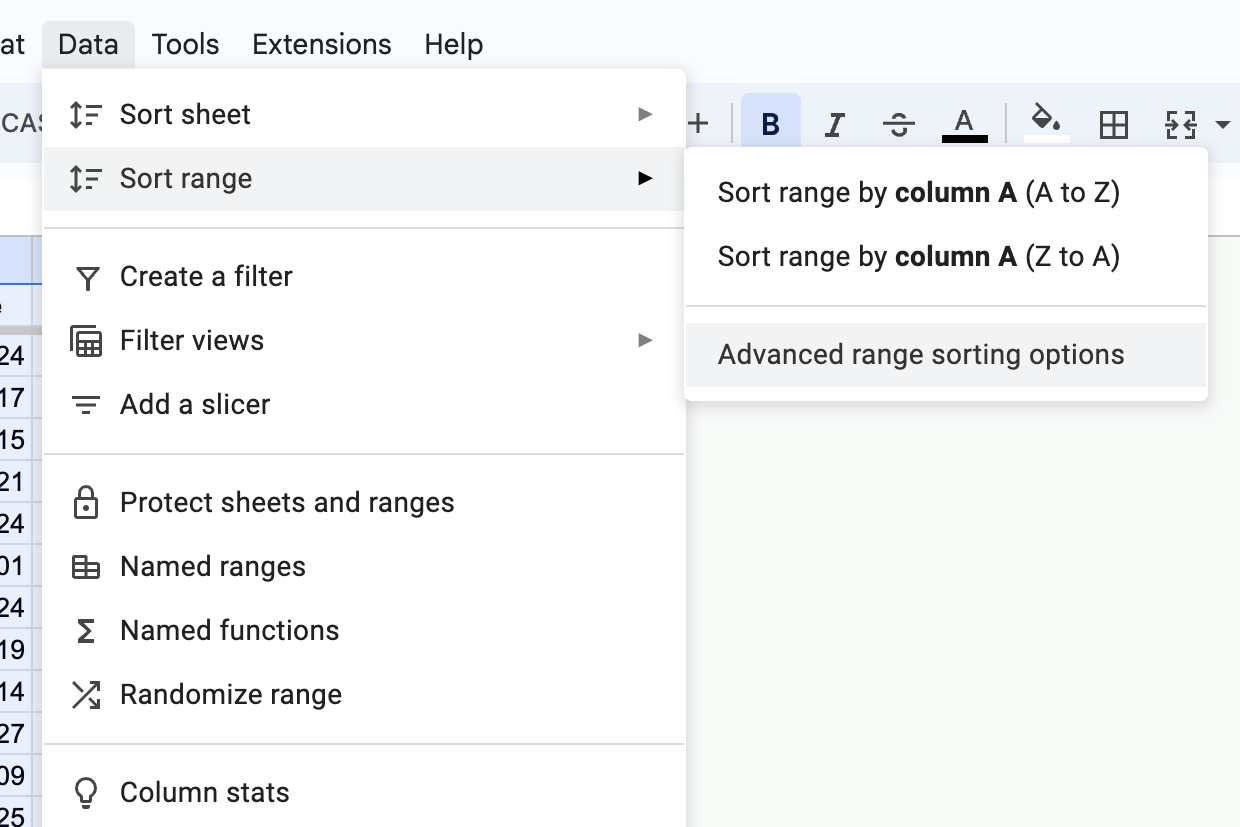
OpenMain Menu -> Data -> Sort range -> Advanced range sorting options.
Open the advanced sort via the main menu
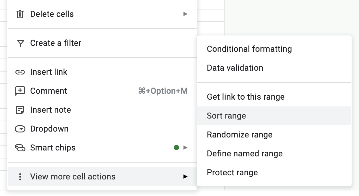
You can get to the same interface via the context menu -> View more cell actions -> Sort range:
Open the advanced sort via the context menu
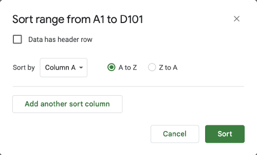
You will see an interface of the advanced sort:
Advanced sort modal window
Check Data has header row (if applicable). It will make selecting the proper columns easier and keep the header row in place.
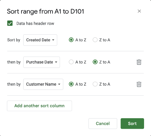
Select the columns by which you need to sort the data and choose the direction.
Sorting by multiple columns with the advanced sort
Click Sort
Sorting with functions works great when you expect the data to change. Google Sheets provides several powerful functions for sorting data.
2. SORT Function
SORT is the most straightforward function for sorting data (documentation):
The SORT function accepts the following arguments:
The range you need to sort. If you provide only this argument, the function will sort it by the first column in ascending order.
The column you need to sort by. It can be either:
the sequential number of a column in the range or
the column outside of the range. It must have the same number of rows as the range being sorted.
The sorting order:
1 or true for ascending,
0 or false for descending.
To sort by multiple columns pass several pairs of column and order arguments:
=SORT(A2:D100,1,false,2,true,4,true)
Please do not pass the header row(s) to SORT: it will be sorted together with all other data.
3. SORTN Function
The SORTN function is very similar to SORT. In addition to just ordering the data, it can limit the output to a given number of columns and take into account relations between the rows (documentation). For example, it works well when you need to output the top N items.
The SORTN function accepts the following arguments:
The range you need to sort. If you provide only this argument, the function will sort it by the first column in ascending order and return the first row.
The number of rows to return. The default is 1.
The display ties mode:
0 (default): return up to N top rows after sorting.
1: return up to N rows plus any rows with the same value in the sort columns as the Nth item.
2: remove duplicates based on the sort columns and return up to N rows.
3: return up to N unique rows based on the sort columns plus all their duplicates.
The column you need to sort by, either:
the sequential number of a column in the range or
the column outside of the range. It must have the same number of rows as the range.
The sorting order:
1 or true for ascending,
0 or false for descending.
To sort by multiple columns pass several pairs of column and order arguments:
=SORTN(A2:D100,10,0,1,false,2,true,4,true)
Please do not pass the header row(s) to SORTN: it will be sorted together with all other data.
4. QUERY Function
QUERY is one of the most powerful functions in Google Sheets. Among other things, you can easily order your data by multiple columns (documentation). Compared to the SORT function above, QUERY has a distinct advantage: it can preserve the header rows in place.
=QUERY(<range>,<query>,[<number_of_headers>])
The function accepts three arguments:
The range can reference to a range or be a constructed array of values.
The query with SQL-like syntax. If you do not provide a query, the function will return the data as is.
The number of header rows (optional) indicates many header rows the data has. If not set or set to -1, the function will try to guess.
Set the number of header rows anyway. QUERY does a great job of guessing the number, but sometimes it can be wrong, and since the function works with dynamic data, it can happen when you are not looking.
The complete query syntax is outside the scope of this guide. These are the basics of the query syntax for sorting data. The query consists of several sections:
SELECT (required): list the columns you want to see in the output or * for all columns. In most cases, you can refer to the columns by their letters (A) or their sequential number in the range (Col1).
WHERE: conditions to filter data. If not provided, QUERY will output all data.
ORDER BY<column_name> [ ASC | DESC ], [ <column_name_2> [ ASC | DESC ], …]: how to order the data. The default order is ASCending if you do not specify otherwise.
For example, this is how you can sort the data by the first and second columns in ascending and descending order respectively, and then output only columns A, B, and C:
=QUERY(Data!A:D,"SELECT A, B, C ORDER BY A ASC, B DESC",1)
or with the sequential column notation:
=QUERY(Data!A:D,"SELECT Col1, Col2, Col3 ORDER BY Col1 ASC, Col2 DESC",1)
Mastering these four sorting techniques in Google Sheets allows you to manage your data more effectively. From the flexibility of the SORT and SORTN functions to the powerful, query-based sorting of the QUERY function, you have various tools at your disposal for any sorting task. Remember, correct data formatting is critical to proper sorting.