7 Ways to Sort Data in Google Sheets

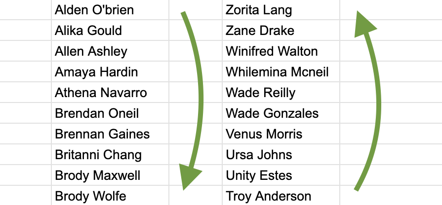
Sorting data in Google Sheets is a common task that can help organize and analyze it. There are multiple ways to order data in Google Sheets, each suitable for different scenarios:

Sort data without functions
     1. Sort Whole Sheet
     2. Sort Selected Range
     3. Advanced Sort of Selected Range
     4. Sort with a Filter
     5. Sort with a Filter View
Sort data with functions
     6. SORT Function
     7. QUERY Function

Using these techniques you can sort by date, alphabet, and number. The advanced sort and SORT / QUERY functions also allow you to sort by multiple columns at the same time.

Sort Without Functions

You can quickly sort data in Google Sheets without functions. It is a good choice when the data is static and you do not expect it to change.

1. Sort the Whole Sheet

To sort the whole sheet by one column, follow these steps:

1. Put your cursor in the column you want to sort the sheet by or select the whole column.
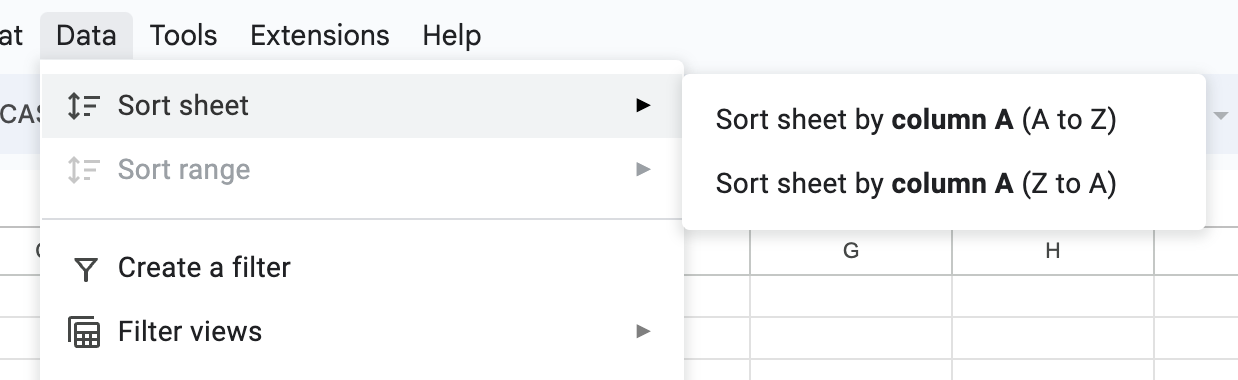
2. Open Main Menu -> Data -> Sort sheet -> Sort sheet by column ... (A to Z) or (Z to A).

   

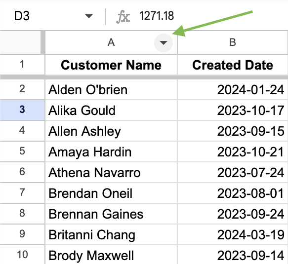
   You can do the same by selecting the whole column and right-clicking or by hovering over the column title and clicking on the triangle that appears there:

   

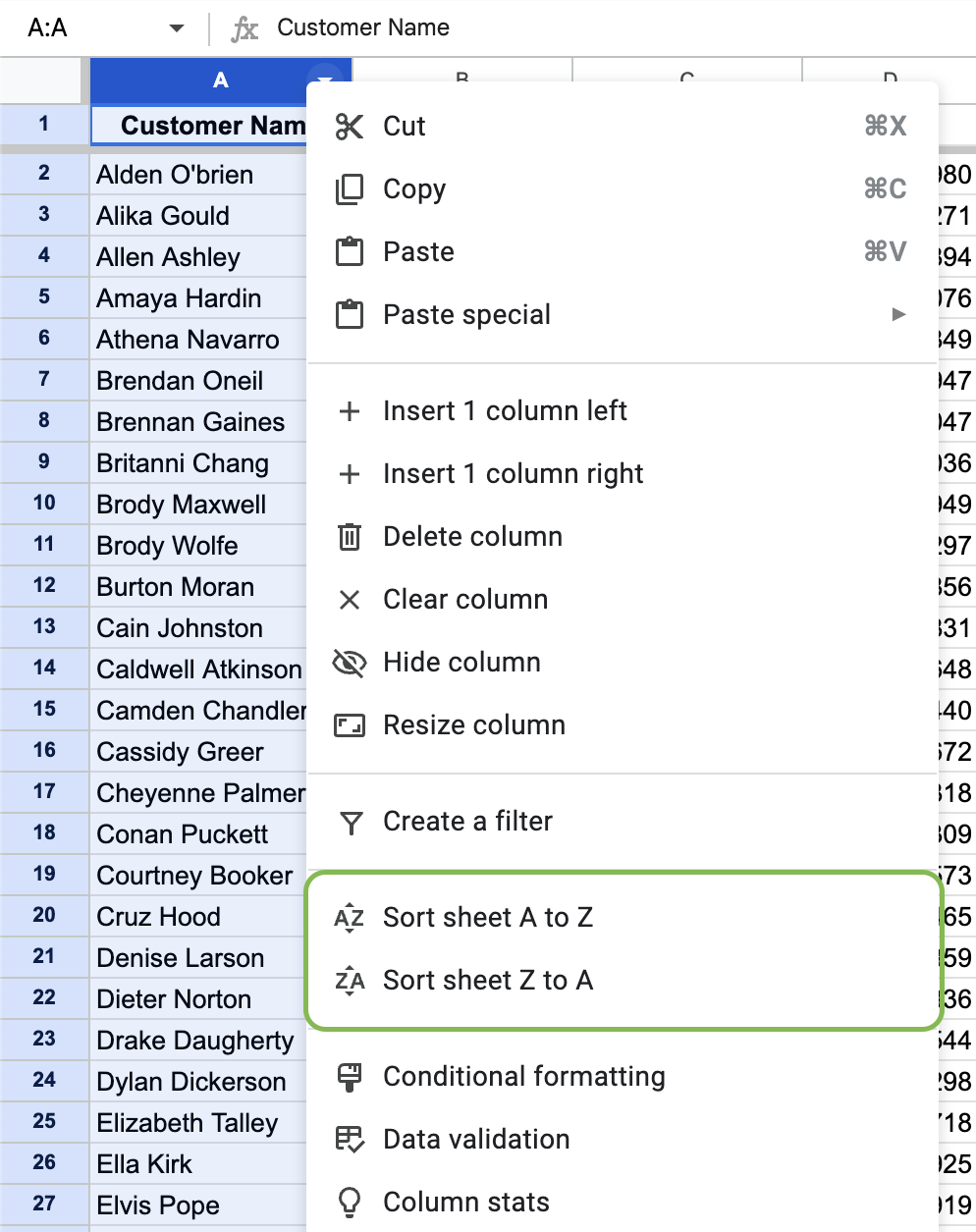
   Then select either of the options to sort the sheet:

   

2. Sort a Selected Range

You can sort a selected range separately from the rest of the sheet. This method works well if you have several data sets on a sheet and want to sort only one.

1. Select the range you want to sort.
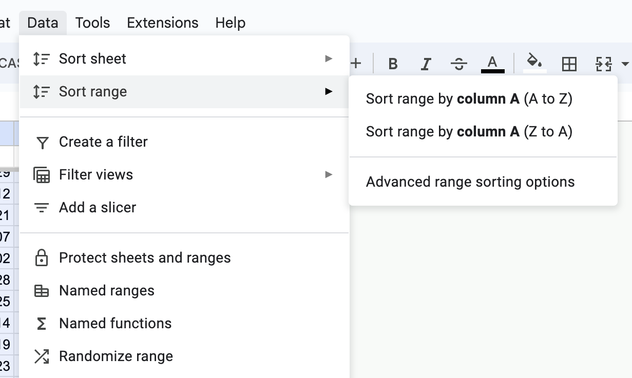
2. Open Main Menu -> Data -> Sort range -> Sort sheet by column ... (A to Z) or (Z to A).

   

3. Advanced Sort and Sort with Multiple Criteria

Google Sheets also allows us to sort a range by multiple criteria (advanced sort). If you select all of it, the sort will apply to the whole sheet.

1. Select the range you want to sort.
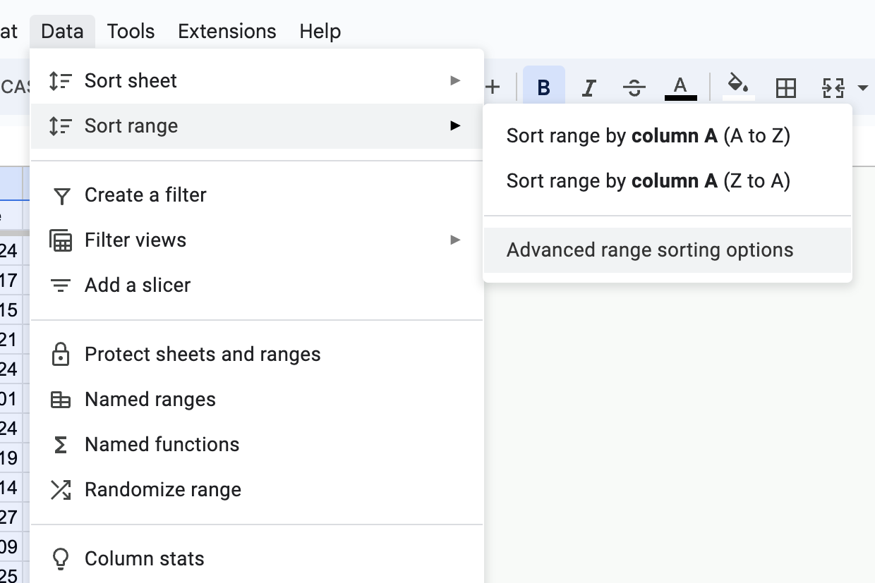
2. Open Main Menu -> Data -> Sort range -> Advanced range sorting options.

   

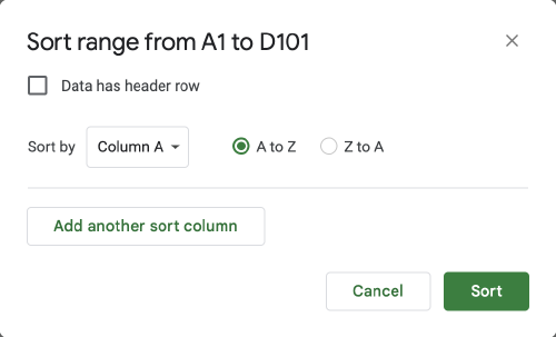
   You will see an interface of the advanced sort:

   

3. Check Data has header row (if applicable). It will make selecting the proper columns easier and keep the header row in place.
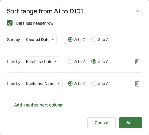
4. Select the columns by which you need to sort the data and choose the order.

   

5. Click Sort

Advanced sort is a powerful feature that allows you to arrange the data in any order you want.

4. Sort with a Filter

You can sort the data using a Filter.

1. Create a filter if you do not have one already:
   1. Select the columns by which you need to sort the data, or do not select anything if you want the filter to apply to the whole sheet.
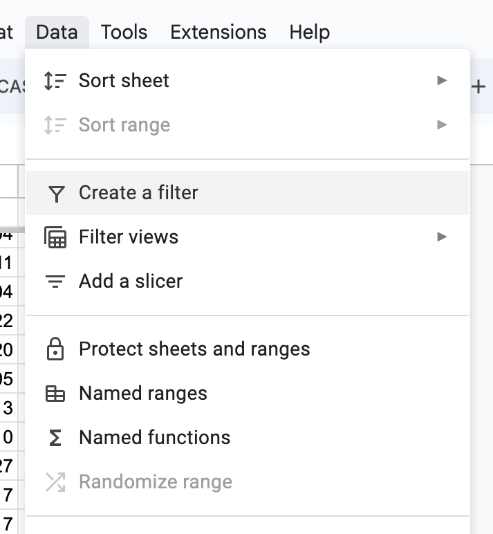
   2. Click Main Menu -> Data -> Create a filter

      

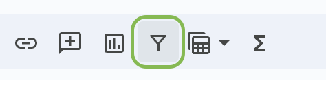
      or use the toolbox:

      

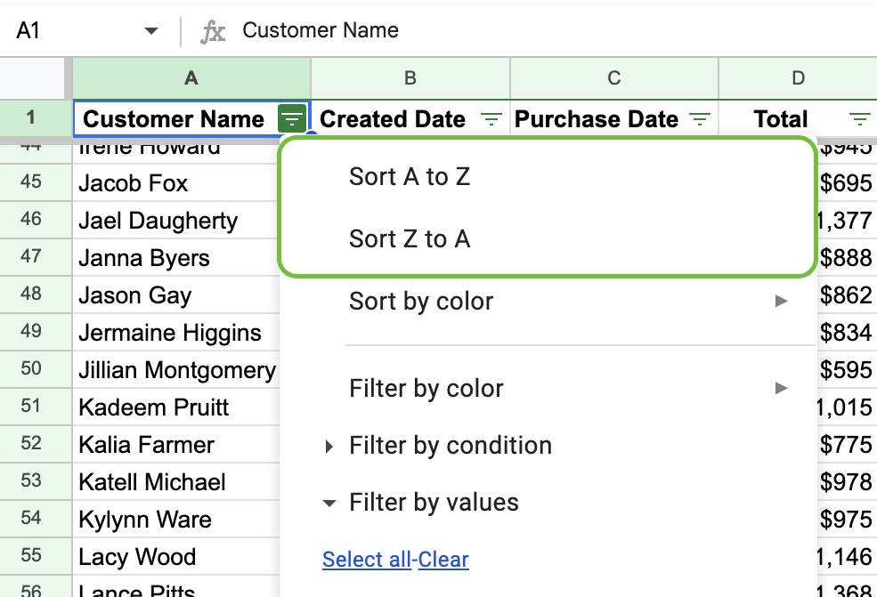
2. Open the header’s menu and select Sort A to Z or Sort Z to A:

   

In all other aspects this method is equivalent to sorting a range or sheet by a given column.

5. Sort with a Filter View

These are the steps to sort data in a filter view:

1. Create a filter view if you do not have one already:
   1. Select the columns you need to sort by, or do not select anything if you want the filter to apply to the whole sheet.
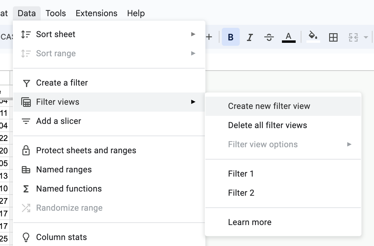
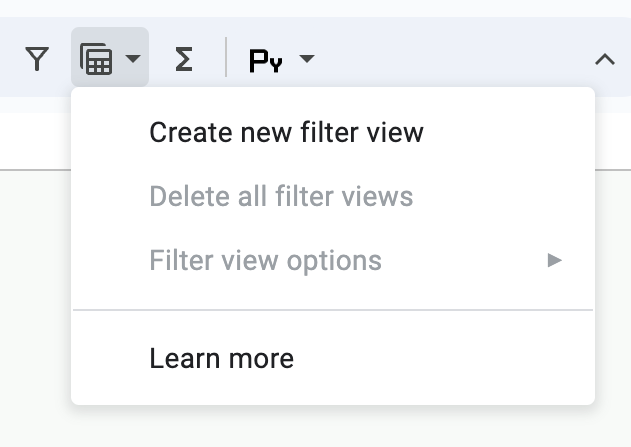
   2. Click Main Menu -> Data -> Filter views -> Create new filter view

      

      or use the toolbox:

      

2. Activate the filter view (if it is not active already).
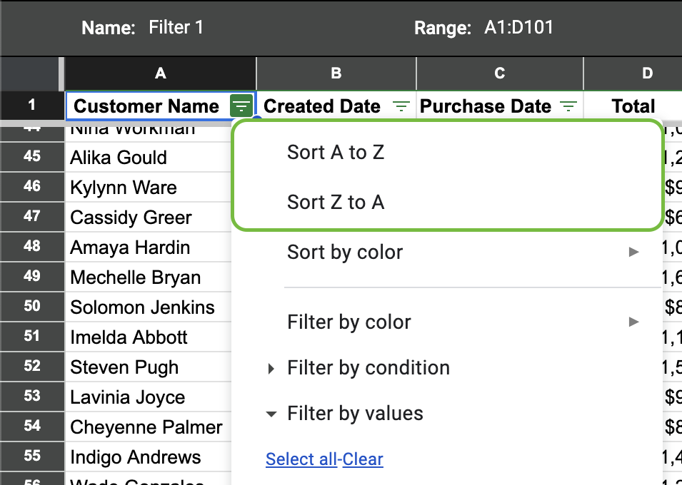
3. Open the header’s menu by clicking the green triangle on the right side of the column header and select Sort A to Z or Sort Z to A.

   

This method is similar to sorting by with a regular filter, with one crucial difference: the changes do not affect the data and are only visible while the filter view is active. It works well for experiments, and when multiple people work on one document and you do not want to interfere with each other.

Sorting With Functions

Sorting with functions works great when you expect the data to change. Google Sheets provides several powerful functions for sorting data.

6. SORT Function

SORT is the most straightforward function to sort data (documentation):

=SORT(
    <range>,
    <sort_column>,
    <is_ascending>,
    [
        <sort_column_2>,
        <is_ascending_2>,
        ...
    ]
)

The SORT function accepts the following arguments:

1. The range you need to sort. If you provide only this argument, the function will sort it by the first column in ascending order.
2. The column you need to sort by, either:
   • the sequential number of a column in the range, or
   • the column outside of the range. It must have the same number of rows as the range.
3. The sorting order:
   • 1 or true for ascending,
   • 0 or false for descending.

To order by multiple columns pass several pairs of a column and order arguments.

Examples:

• Sort by the first column of the data range in ascending order:
  =SORT(A2:D100), equivalent to =SORT(A2:D100, 1, true)
• Sort by the second column in the range in descending order:
  =SORT(A2:D100, 2, false)
• Sort by multiple columns in different orders:
  =SORT(A2:D100, 1, false, 2, true, 4, true)
• Sort by an external column:
  =SORT(A2:D100, E2:E100, false)

Google Sheets also supports the SORTN function, which, in addition to sorting, can limit the output to a given number of columns and can take into account relations between the rows (documentation).

7. QUERY Function

You can easily sort data with the QUERY function, including complex sorting by multiple columns (documentation). Compared to the SORT function above, QUERY has a distinct advantage: it can preserve the header rows in place.

=QUERY(
    <range>,
    <query>,
    [<number_of_headers>]
)

The function accepts three arguments:

1. The range can be a reference to a range or a constructed array of values.
2. The query with SQL-like syntax. If you do not provide a query, the function will return the data as is.
3. The number of header rows (optional) indicates many header rows the data has. If not set or set to -1, the function will try to guess.

The complete query syntax is outside the scope of this guide. These are the basics of the query syntax for sorting data. The query consists of several sections:

1. SELECT (required): list the columns you want to see in the output or * for all columns. In most cases, you can refer to the columns either by their letters (A) or their sequential number in the range (Col1).
2. WHERE: conditions to filter data. If not provided, QUERY will output all data.
3. ORDER BY <column_name> [ ASC | DESC ], [ <column_name_2> [ ASC | DESC ], …]: how to order the data. The default order is ASCending if you do not specify otherwise.

Here are some examples of how to sort data with the QUERY function (assuming that the data is in Data!A:D):

• Sort by the first column in descending order:
  =QUERY(Data!A:D, "SELECT * ORDER BY A DESC", 1) or
  =QUERY(Data!A:D, "SELECT * ORDER BY Col1 DESC", 1) with the sequential column notation.
• Sort by the first and second columns in ascending and descending order respectively, and then output only columns A, B, and C.
  =QUERY(Data!A:D, "SELECT A, B, C ORDER BY A ASC, B DESC", 1) or =QUERY(Data!A:D, "SELECT Col1, Col2, Col3 ORDER BY Col1 ASC, Col2 DESC") with the sequential column notation.

Selecting the appropriate method depends on the specific needs of your task, such as whether you need a dynamic solution that updates automatically (like the SORT and QUERY functions) or a manual method that offers immediate, straightforward sorting (like using the menu options or filters).