How to Version Data in Google Sheets
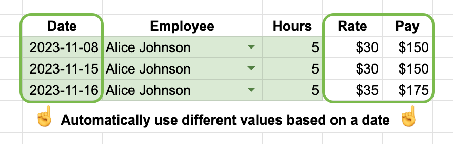
One of the most challenging parts of Google Sheets is working with changing values while preserving their history, also known as versioning. Let’s say you have a team of employees paid by hour based on their hourly rate. You keep all rates in the Employees sheet.

You record how much they worked each day in the Hours sheet, and pull the appropriate rate from the Employees sheet with a VLOOKUP or XLOOKUP function:
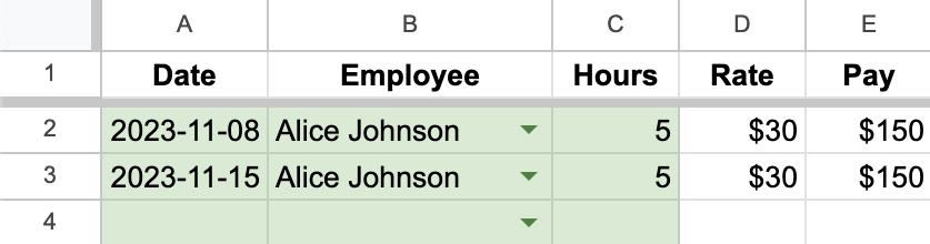
To improve the usability of the sheet, we indicate a range that must be edited manually with a green background.
Then, in some other sheet, you calculate weekly/monthly pay.
However, there is a problem: with this setup, you cannot store the history of the rates throughout time and apply them to corresponding periods. For example, you need to change somebody’s hourly rate starting tomorrow. If you change the rate in place, it will also apply to previous periods. Sometimes, it is not a problem, but more often than not, we want to preserve the history, at least for analytics and reporting purposes.
There is a reasonably easy way to do it, but it will require some work. This method can be applied to any situation when you need to preserve and use the history of changes in different places. Let’s break it down step by step. You can find a working example in this spreadsheet.
1. Add “Effective From” Column
The first step is to add an Effective From column to the Employees sheet. It will indicate the first day when this rate will start applying:
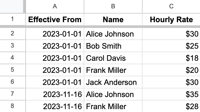
You can add a calendar dropdown to simplify working with the effective date.
2. Create an Intermediary Sheet with Sorted Data
Then, you need to create an intermediary sheet where we will sort the data by the effective date in reverse chronological order: from the newest to oldest. It is necessary for the next step.
=SORT({'Employees'!A2:C}, 1, false)
This formula takes all employee data rows (excluding the header row) and sorts them by the effective date in descending order.

To distinguish the Employees sheet from this intermediary sheet, you can call it employees_pr and hide it later. Starting the name with a lowercase letter indicates that you do not need to edit this sheet manually, employees part means that it is related to the Employees sheet, and pr shows that it is “processed.”
3. Modify Rate Lookup Formula
Finally, we need to create a function to fetch the proper rate based on a date and name:
=INDEX(
    FILTER(
        employees_pr__rate,
        employees_pr__name=B4,
        employees_pr__eff_from<=A4
    ),
    1,
    1
)
To make the formula more readable, we used named ranges. Read more on what named ranges are, how to create them, the top 7 advantages of using named ranges, and best naming and sizing practices.
Let’s break down how it works:
-
FILTERgets all rates that conform to two requirements:- has a particular employee name, and
- effective date is less or equal to the reference date
As a result,
FILTERreturns all rates that came into force before or on the reference date. -
INDEXreturns the first rate. Since we sorted the rates from newest to oldest in Step 2, the first rate will be the one that applies on the reference date.
You can also use the IFNA function to provide a fallback value instead of a #N/A error.
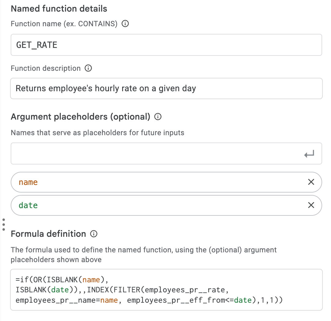
4. Optional: Create a Named Function
You can convert the formula from Step 3 into a named function to reduce repetition. This way, if you have to change anything, you will need to do it only in one place.
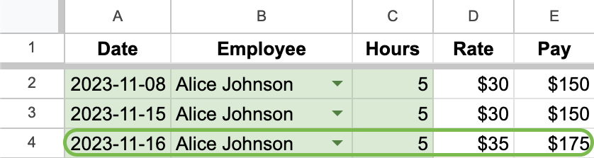
Now the formula on the Hours sheet looks much better:
=MAP(A2:A, B2:B, LAMBDA(date, name, GET_RATE(name, date)))
To avoid repeating the function in each row, we used the MAP function to loop through all rows and run GET_RATE to get the appropriate hourly rate.
We hope this guide helps you with versioning your data in Google Sheets. By following these steps, you can preserve the history of your data and use it in different places without worrying about losing the accuracy of your calculations.