Flexible and Extensible Color-Coding System in Google Sheets

When you’re faced with an abundance of information, color-coding can make it easier to quickly discern when something demands your attention. Google Sheets’ conditional formatting can prove immensely helpful here, enabling you to alter the appearance of a cell depending on its content.

However, the standard conditional formatting is static, requiring you to change the rule itself to adjust a threshold or other conditions. While this is relatively straightforward with a few coloring rules, it becomes more challenging when you have numerous rules or need to make dynamic adjustments.

A more effective approach involves moving the thresholds and other rules to a separate settings page and referencing them in conditional formatting’s custom formulas. This will allow you to:

• Adjust formatting rules on the fly, without having to directly modify the conditional formatting.
• Make the document easier to maintain and expand.

In this post, we’ll explore an example of how to highlight cells based on the color group associated with their content.

Coloring Groups

Suppose we have a limited set of values that can be classified into several groups, such as order, task, project statuses, etc. Using a traffic light analogy, we could have three types of statuses:

• 🔴 Red: Requires attention or correction (complaint, return, cancellation).
• 🟡 Yellow: Needs monitoring to prevent escalation to red (delay, failed delivery).
• 🟢 Green: Everything is proceeding as planned (received, scheduled for delivery, completed).

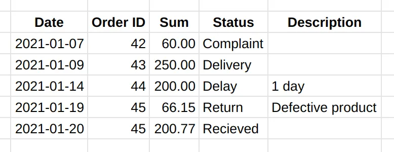
Before we apply conditional formatting it can look like this:

There are multiple ways to achieve this in Google Sheets, and your choice will depend on the specifics of your use case (complexity of coloring rules, etc.). In this post, we’ll create a simple setup with the COUNTIF() formula and a settings page with easily modifiable coloring rules. This is ideal when you need to color cells whose content matches a particular value, and you plan to use a small number of colors.

Our setup will comprise three components: settings sheets, named ranges, and conditional formatting formulas.

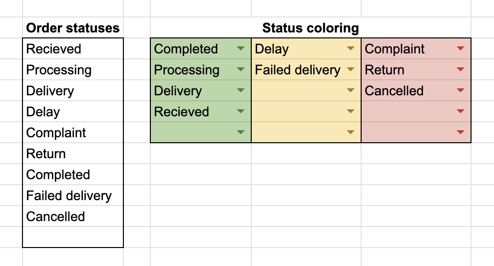
1. Settings Sheet

The process of setting up coloring rules begins with a settings area where you will define what gets colored and which color to use.

• Create a separate Settings sheet (name is arbitrary). Keeping settings distinct from the data leads to more robust and flexible spreadsheets.

• Compile a comprehensive list of all values that will be used to determine the color. In our example, this would be the status of an order, but in your case, it could be anything else.

• Create three sections for each color group: red, yellow, and green, for example, by segregating them into separate columns.

• Optionally, you could use data validation to create dropdowns in each of the sections based on the total list of statuses.

Eventually, you should have something akin to this:

2. Named Ranges

To link the conditional formatting to the rules we just established, we need to create named ranges. In accordance with best naming practices, we’ll generate one for each of the coloring rules:

• sett_coloring_red
• sett_coloring_yellow
• sett_coloring_green

3. Conditional Formatting

Finally, we need to establish conditional formatting rules that incorporate these settings and named ranges.

• Select the range containing statuses (e.g., the entire column).
• Right-click ➞ Conditional Formatting ➞ Add another rule (it may open automatically).
• Format cells if … ➞ Custom Formula is
• Apply the following formula: =COUNTIF(INDIRECT(“[RANGE_NAME]”), [STARTING_CELL]), where:
  • [RANGE_NAME] is the name of the colored range you intend to use.
  • [STARTING_CELL] is the reference to the top-left cell of the range to which you’re applying the conditional formatting.

For example, if the named range is sett_coloring_green and the rule is applied to D2:D1000, the formula would look like this:

1=COUNTIF(INDIRECT(“sett_coloring_green”), D2)

Here’s how it works. The COUNTIF() function accepts two parameters:

1. The range where it will search for the occurrence of the search value. In this case, we use the function INDIRECT(“sett_coloring_green”), which returns a reference to the range specified in the quotes. Regrettably, you can’t directly refer to a named range (or to a regular range outside the current sheet) in conditional formatting.

2. The search value, which is the cell containing a status we want to color. Here we set the top-left cell of the range to which we’re applying conditional formatting. Google Sheets will automatically adjust the reference behind the scenes.

This custom formula counts how many times the cell value (which contains the status to be colored) appears in the coloring settings range. If everything is set up correctly, this will be either 1 or 0, which will be interpreted by the conditional formatting as true or false, thereby enabling or disabling the formatting.

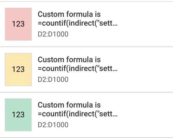
Now we need to create two more conditional formatting rules for the other colors. We should end up with the following rules. Their order doesn’t matter here, as only one should be active at any given time:

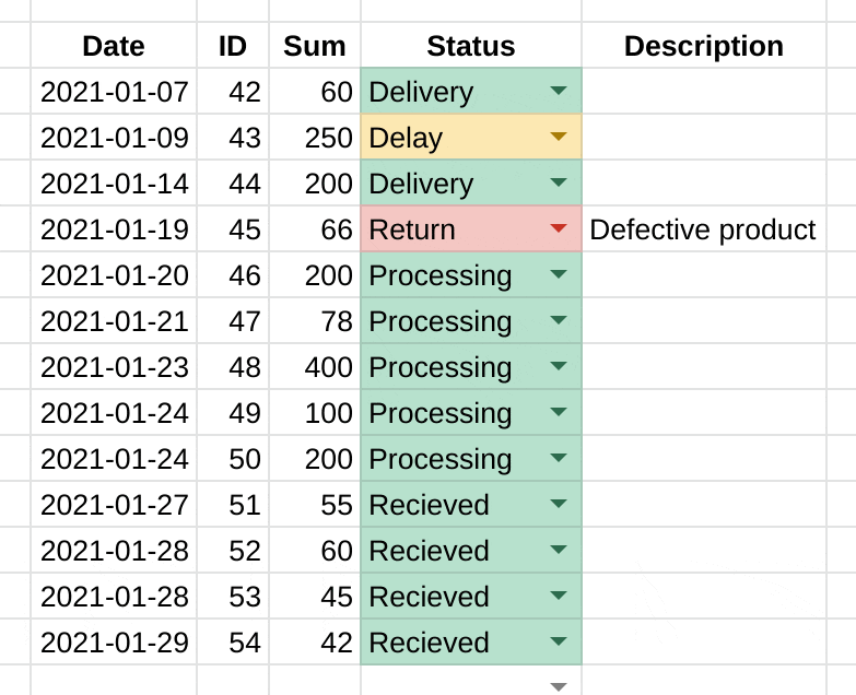
It’s now ready: all statuses defined in the coloring rules are now color-coded accordingly.

With the skills you’ve acquired in setting up a robust and flexible color-coding system in Google Sheets, your data analysis will be both more efficient and more insightful. Not only have you made your spreadsheets more visually engaging, but you’ve also built a system that’s extensible, capable of growing and adapting to your future data needs.