Practical Solutions for IMPORTRANGE "Result too large" Error
One of the most common issues with IMPORTRANGE in Google Sheets is the “Result too large” error. In this post we will cover different aspects of dealing with it:
What Causes “Result too large” Error
General Recommendations
How to deal with the error:
1. Copy Data Manually
2. Importing All Chunks One by One
Optional Improvement: Use IFERROR and Named Ranges
3. Combine Manual Copying with IMPORTRANGE
4. Array Literals
5. Import Chunks with VSTACK
Optional: Make the Formula More Robust
6. Import Row by Row
7. Automatically Import All Data with One Formula
Optional: Use Named Functions
What Causes “Result too large” Error
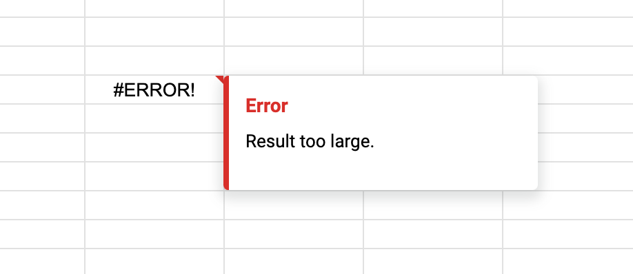
According to Google’s documentation, this error occurs when the data you import exceeds 10 MB. The practical implications of this limit depend on the number of cells and the volume of data they contain.
A general guideline is to import between 50,000 to 100,000 cells per IMPORTRANGE formula; this number should be lower if the cells are data-heavy. For instance, if your range includes ten columns, you might limit your import to 10,000 rows.
To circumvent the “Result too large” error, you can employ formulas or Google Apps Script. In this post we will focus on formula-based solutions, which typically involve segmenting the data into smaller portions and importing these individually. The method you choose will depend on your specific needs, such as the amount of data, whether it is expected to grow, how often it changes, and your personal preference.
Word of caution: While the techniques below can import much more data than a standalone IMPORTRANGE, they may affect spreadsheet performance, especially if the imported data updates frequently. Excessive use might also lead to throttling of your requests. In these cases, using Apps Script to move data around makes sense.
General Recommendations
If you’re facing the “Result too large” error, consider the following tips:
- Only import the data you need; exclude unnecessary rows and columns you don’t use in the target document.
- Perform as much data processing as possible in the source document.
- Assess whether using formulas to import data is feasible. Sometimes, Apps Script may be a better solution.
We will go from the least to the most complex methods.
1. Copy Data Manually
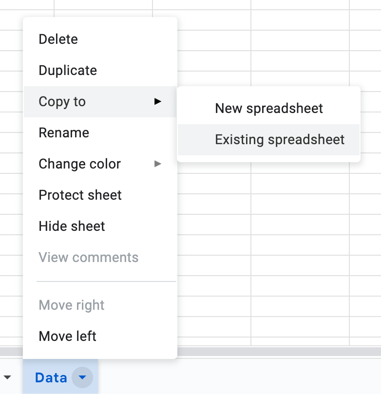
The least appealing way to transfer a lot of data between spreadsheets is to manually copy it, either with regular copy-paste or by copying the sheet with data from the source to the target spreadsheet:
This is a very low-tech solution; you can achieve the same with other methods below. However, there is an actual use case when this is arguably the best approach (on par with copying via Apps Script):
- You have a lot of data: millions of cells or hundreds of megabytes.
- The data is updated very infrequently, for example, monthly. Or you analyze data with the same cadence.
In these cases, it often makes sense to transfer the data manually. Caveat: if you copy the entire sheet, you will need to adjust how other formulas consume this data because, in most cases, just renaming sheets will not work. My go-to solution is using named ranges and simply changing which sheet they target — more on the advantages of using named ranges.
2. Importing All Chunks One by One
Another relatively low-tech solution is to import chunks one by one in several IMPORTRANGE functions, spacing them on the sheet accordingly. For example, if you import chunks of 10,000 rows, you will put a similar formula in the first row:
=IMPORTRANGE("<url or id>", "Data!A1:H10000")
Then, in row 10,001, you will import the second chunk:
=IMPORTRANGE("<url or id>", "Data!A10001:H20000")
Rinse and repeat as many times as you need.
This method requires more effort; however, it works well in one case:
- You have a lot of data: millions of cells or hundreds of megabytes.
- The data is only appended, and previous rows are not changed. This means that only the latest
IMPORTRANGEwill get updated on each change, which will reduce the overall load on the spreadsheet and usually make it faster.
Optional: Use IFERROR and Named Ranges
We can improve the formula above in two ways:
- Wrap it in
IFERRORto provide retry logic. Sometimes,IMPORTRANGErandomly fails, and it doesn’t always recover from it on its own. - Use named ranges for repeated values: source document url/id and sheet name. This way, it will be trivial if you need to change the source in the future.
The updated formula will look something like this (using the recommended naming convention for ranges):
=IFERROR(
    IMPORTRANGE(sett__source_sheet_url, sett__source_sheet_name&"!A1:H10000"),
    IMPORTRANGE(sett__source_sheet_url, sett__source_sheet_name&"!A1:H10000")
)
You could convert it into a named function if you have many chunks.
3. Combine Manual Copying with IMPORTRANGE
If you have a lot of data and it is only appended, you could also combine methods #1 and #2:
- Manually copy the static part of the data to the target sheet. For example, rows 1 to 100,000.
- Use
IMPORTRANGEto import the range where data is being appended, rows from 100,001. - Extend the static part of the data as required, shifting the formula with
IMPORTRANGE.
4. Array Literals
Before VSTACK and HSTACK were added to Google Sheets (more on them below), array literals were the primary method of joining multiple chunks of data, including several IMPORTRANGE:
={
    IMPORTRANGE("<url or id>", "<range, part 1>");
    IMPORTRANGE("<url or id>", "<range, part 2>");
    IMPORTRANGE("<url or id>", "<range, part 3>")
}
This approach will stack the results of each IMPORTRANGE on top of each other. The main drawback of this approach is that these ranges must have the same number of columns; otherwise, the whole formula will return an “Array Literal was missing values for one or more rows” error:
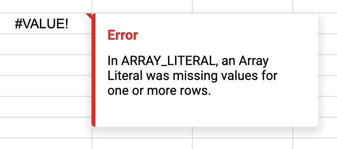
Array literals’ strictness can also be beneficial if you need to enforce data integrity and “fail fast” when the number of columns does not match.
5. Import Chunks with VSTACK
A more convenient way of importing data in chunks is using VSTACK. The simplest option looks like this:
=VSTACK(
    IMPORTRANGE("<url or id>", "<range, part 1>"),
    IMPORTRANGE("<url or id>", "<range, part 2>"),
    IMPORTRANGE("<url or id>", "<range, part 3>")
)
Each IMPORTRANGE will import a part of the data, and VSTACK will stitch them on top of each other. If you split data by columns, you can do the same with HSTACK.
The ranges can have different numbers of columns (rows for HSTACK), and the result will still be imported; wrap the function in IFERROR that will remove missing data warnings.
Optional: Make the Formula More Robust
The formula above suffers from two drawbacks:
- You have to repeat the spreadsheet url and sheet name many times. (which makes it more error-prone to change).
- It does not handle possible
IMPORTRANGEerrors at all. They are rare but still happen and are hard to track down if you do not think about it in advance.
This formula fixes this issue (see breakdown below):
=LET(
    url,
    "<spreadsheet url or id>",
    sheet_name,
    "<name of the source sheet>",
    VSTACK(
        IFERROR(
            IMPORTRANGE(url, sheet_name&"!A1:H10000"),
            IMPORTRANGE(url, sheet_name&"!A1:H10000")
        ),
        IFERROR(
            IMPORTRANGE(url, sheet_name&"!A10001:H20000"),
            IMPORTRANGE(url, sheet_name&"!A10001:H20000")
        ),
        IFERROR(
            IMPORTRANGE(url, sheet_name&"!A20001:H30000"),
            IMPORTRANGE(url, sheet_name&"!A20001:H30000")
        )
    )
)
The formula might look complex, but everything here has a purpose. Let’s break it down:
- In the first four arguments of the
LETfunction, we create url and sheet_name variables. This way, we can set them once and reuse them in subsequent functions without repeating them. Having done that, we can easily change the source document or sheet later. - The last argument of the
LETfunction is the function that uses those variables –VSTACK. It vertically stacks all data from the functions inside of it. - Inside
VSTACK, we run multipleIMPORTRANGEfunctions for different data chunks. - We repeat each
IMPORTRANGEtwice inside theIFERRORfunction to allow for error handling. If the firstIMPORTRANGEfails (which happens sometimes), it will be called the second time. Without it, you may miss one of the data segments without noticing it.
6. Import Row by Row
Another way to avoid IMPORTRANGE’s “Result too large” error is to import all data row by row:
=MAP(
    SEQUENCE(<number of rows>),
    LAMBDA(
        row,
        IMPORTRANGE("<url>", "<source sheet name>!"&row&":"&row)
    )
)
This is how it works:
SEQUENCEgenerates a list of numbers from 1 to a given number of rows. You need to set this number manually or calculate it in the source document and import it separately.MAPgoes through these numbers one by one and passes them toLAMBDAas a row.LAMBDAuses the row to callIMPORTRANGEto import a given row.MAPcombines responses fromLAMBDAs and outputs them to the given spreadsheet.
It might look like the spreadsheet will call IMPORTRANGE as many times as you have rows; however, it batches the requests under the hood, and their actual number is much smaller.
7. Automatically Import All Data with One Formula
The weak spot of the above approach is that you have to manage all the chunks and their size manually. We can automate it with this formula (see breakdown below):
=LET(
    url,
    "<spreadsheet url or id>",
    sheet_name,
    "<name of the sheet>",
    first_col,
    "<letter of the first column to be imported>",
    last_col,
    "<letter of the last column to be imported>",
    total_rows,
    10000,
    rows_per_chunk,
    200,
    REDUCE(
        "initial_value",
        MAP(
            SEQUENCE(ROUNDUP(total_rows/rows_per_chunk), 1, 1, rows_per_chunk),
            LAMBDA(row_num, sheet_name&"!"&first_col&row_num&":"&last_col&(row_num + rows_per_chunk - 1))
        ),
        LAMBDA(
            results,
            range_name,
            LET(
                result,
                IFERROR(
                    IMPORTRANGE(url, range_name),
                    IMPORTRANGE(url, range_name)
                ),
                IF(
                    results="initial_value",
                    result,
                    VSTACK(results, result)
                )
            )
        )
    )
)
Let’s break it down step by step:
- We define several variables that we will use later with the
LETfunction. It is not strictly necessary, but it helps with managing all options in one place:- url: url or id of the source spreadsheet
- sheet_name: name of the source sheet
- first_col: letter of the first column in the range we need to import
- last_col: letter of the last column in the range we need to import
- total_rows: total number of rows we need to import
- rows_per_chunk: how many rows to import per chunk of data; the source sheet should have at least the number of chunks x rows_per_chunk number of rows; otherwise some of the imports will fail
- The
REDUCEfunction allows us to run other functions multiple times and aggregate the result. It accepts three arguments:-
Initial value of the so-called “accumulator” – this is the variable we will use to store intermediate values after each iteration. Here, we use the string “initial_value” to account for a special case of the first chunk.
-
The list of values
REDUCEwill iterate over. Here,MAPgenerates a list of ranges that we will need to import:ROUNDUP(total_rows/rows_per_chunk)calculates the number of data chunks we need to import.SEQUENCE(ROUNDUP(total_rows/rows_per_chunk), 1, 1, rows_per_chunk)generates starting row number for each chunk- This list is passed to
LAMBDA, which concatenates sheet_name, first_col, and last_col and generates the proper ranges we will import.
-
A function that accepts the accumulator and a value from the list of values and returns an updated accumulator (it will be passed to the next run of this function). This function will run as many times as there are values in the list.
LAMBDAfunction imports each chunk of data. As usual, we wrap eachIMPORTRANGEinIFERRORto allow for retries. We call imports insideLETsolely to avoid duplicating imports.The first chunk is a special case: the accumulator is initiated to an arbitrary “initial_value” as the first time we do not have anything to append data to, and
LAMBDAreturns the first chunk that becomes the base for appending data in later iterations.
-
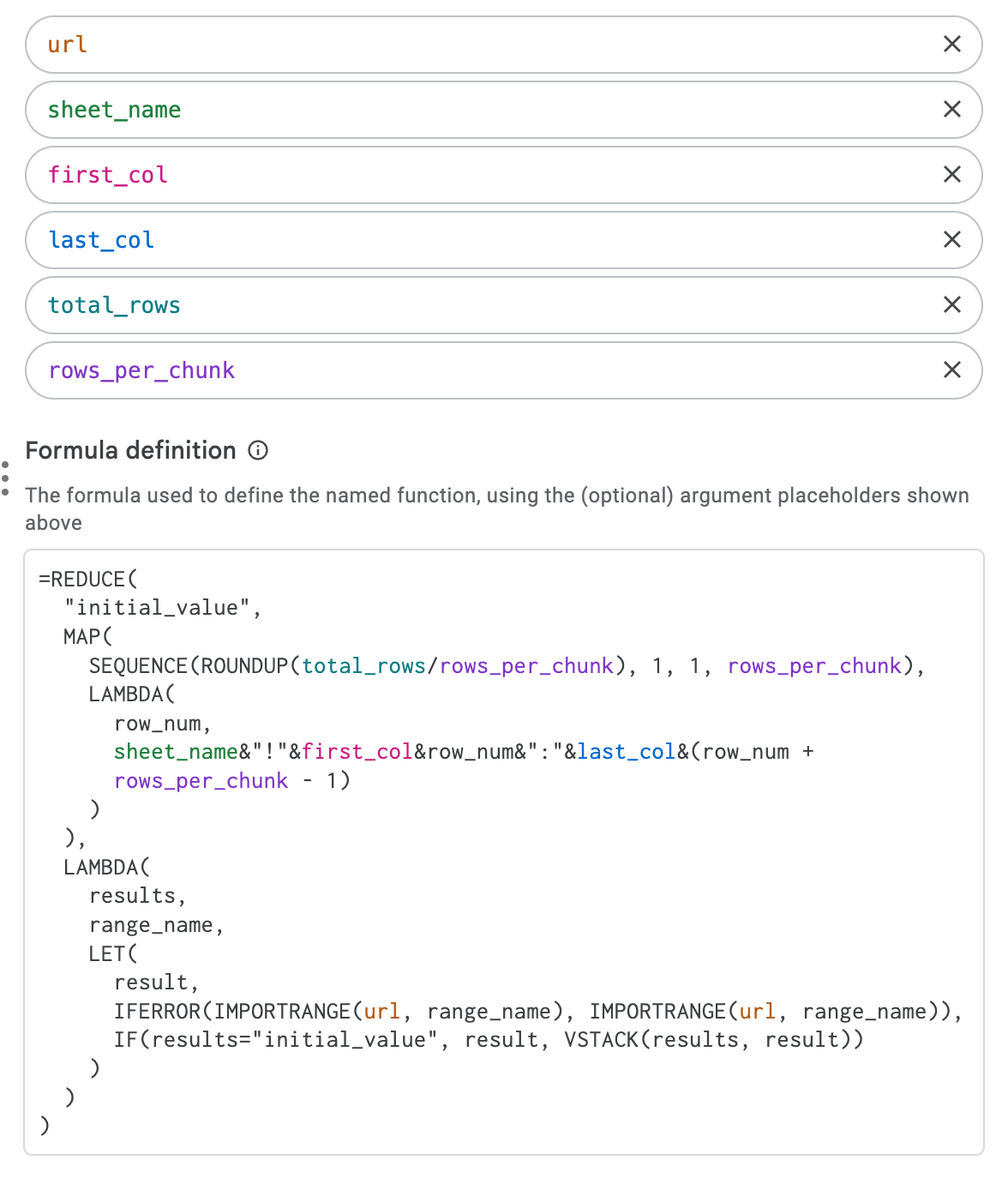
Optional: Use Named Functions
You can easily convert this formula into a named function that will be easy to use:
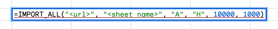
The function itself will also be shorter since we do not need to use the first LET:
=REDUCE(
  "initial_value",
  MAP(
    SEQUENCE(ROUNDUP(total_rows/rows_per_chunk), 1, 1, rows_per_chunk),
    LAMBDA(
      row_num,
      sheet_name&"!"&first_col&row_num&":"&last_col&(row_num +
      rows_per_chunk - 1)
    )
  ),
  LAMBDA(
    results,
    range_name,
    LET(
      result,
      IFERROR(IMPORTRANGE(url, range_name), IMPORTRANGE(url, range_name)),
      IF(results="initial_value", result, VSTACK(results, result))
    )
  )
)
Below is the complete setup of the named function:
By now, you should have a robust understanding of the various strategies to bypass the “Result too large” error in Google Sheets. Remember, whether it’s segmenting data for selective importing, leveraging formulas, or employing Google Apps Script, the key is to choose the method that best suits the scale and dynamics of your data.